Climate Feedbacks and Climate Sensitivity

Forcing and Response

We’ve learned that the climate system can be forced by external processes. For example, the Earth’s temperature is partly determined by the Sun’s energy output. We call this a ‘radiative forcing’. Changes in forcing are due to changes in external, but not internal, processes. Internal processes are those that occur within the climate system itself. Examples include weather systems, ocean circulations, and land-surface processes. External processes are unaffected by the state of the system. As an example, the flow of energy from the Sun is unaffected by the state of the Earth’s climate system. Note that even though human affairs are strongly affected by climate, human activities, such as the emission of greenhouse gases, are considered ‘external’ to the climate system.

Consider a simple example. Suppose that the brightness of the Sun were to change. This would produce a response or change in the Earth’s temperature. We can capture this idea mathematicallyThe following derivation follows that in: Roe, Feedbacks, Timescales, and Seeing Red, (2009). Please see this source for further details. by writing that for a given change in radiative forcing, \(\Delta R\), there will be a change in temperature, \(\Delta T\), such that \[\lambda \Delta R = \Delta T \; , \tag{1}\] where \(\lambda\) is called the climate sensitivity parameter, which determines how strong the temperature response is for a given climate system. This equation is a ‘linear’ equation and assumes that the change in forcing, \(\Delta R\), is relatively small (the current energy imbalance due to global warming is about 1 \(\text{W}/\text{m}^2\), compared to the total energy flux of about 340 \(\text{W}/\text{m}^2\)).

The most fundamental planetary energy balance we can use in calculating the climate sensitivity parameter, \(\lambda\), is the Stefan-Boltzman law, \(\mathcal{F}=\sigma T^4\), that we learned about in Chapter 2. We can write Eq. (1) in differential form, plug in the Stefan-Boltzman law, and take its derivative to get the following, \[\lambda = \frac{\Delta T}{\Delta R } = \frac{dT}{dF} = \frac{1}{dF/dT} = \frac{1}{4\sigma T^3} \; .\] In Chapter 2 we calculated that the Earth without an atmosphere would be 253.7 K, so this implies that \(\lambda = 0.27\,\text{m}^2\text{K}/\text{W}\) for the most fundamental energy balance model of Earth. What does this value of \(\lambda\) mean? It means that for every 1 \(\text{W}/\text{m}^2\) of excess radiative forcing, our modeled planet will increase its temperature by 0.27 K.

So Eq. (1) works for a planet with no atmosphere. But what if by changing the solar radiative forcing, the Earth’s atmosphere were to respond in some way? What if the atmosphere could counteract or damp the forcing? If the Sun were to put out more energy, perhaps the Earth’s atmosphere could change somehow to cool itself down so that it wouldn’t warm as much as it might otherwise do without an atmosphere? Alternatively, perhaps it’s possible for Earth’s atmosphere to amplify the increase in solar radiation, making Earth even hotter than it might otherwise be? These effects are called ‘feedbacks’ and they occur widely in many technical fields and even in daily life. ‘Positive feedbacks’ amplify and ‘negative feedbacks’ counteract or damp.

A familiar example of a positive feedback is the unpleasant squeal produced by a sound system that includes a microphone, an audio amplifier, and a speaker.These examples are from: Randall, Atmosphere, Clouds, and Climate, (2011). A sound picked up by the microphone is amplified and played through the speaker. If the speaker is too close to the microphone or if the gain of the amplifier is turned up too high, the sound produced by the speaker is picked up by the microphone and further amplified, leading to the familiar screeching of audio feedback. Small perturbations are amplified; this is characteristic of a positive feedback.

A familiar example of a negative feedback is temperature control by a thermostat that is coupled to a heating, ventilation, and air conditioning system. After you set a target temperature, the thermostat detects temperature excursions from the target value and commands the system to fight against those excursions by warming when the room is too cool and cooling when the room is too warm. Small perturbations are damped; this is characteristic of a negative feedback.

How then can we add feedbacks into our mathematical description of climate forcing, Eq. (1)? Adding in a feedback means that some part of the temperature response gets ‘fed back’ or added back into the radiative forcing; some of the temperature ‘output’ is fed back into the radiative ‘input’, so that it can increase or reduce the effect of the initial forcing. The simplest representation of this small radiative addition is linear, \(c_1 \Delta T\), where \(c_1\) is the proportion of the temperature response that affects the radiative forcing. So we can modify Eq. (1) so that we have \[\Delta T = \lambda (\Delta R + c_1 \Delta T )\; ,\] and solving for \(\Delta T\) we have \[\Delta T = \frac{\lambda \Delta R}{1-c_1\lambda} \; .\] This equation is often simplified slightly by introducing the ‘feedback factor’ \(f=c_1\lambda\), so that \[\Delta T = \frac{\lambda \Delta R}{1-f} \; . \tag{2}\]

Mathematically, a negative feedback means that \(f\) is negative, while a positive feedback means that \(f\) is positive. If there are no feedbacks, and thus \(f=0\), then we get back our initial Eq. (1). If we have several different feedbacks, these can just be added into \(f\) because they too are just additions or subtractions to the radiative change (e.g., for three feedbacks \(f=f_1+f_2+f_3\)).

It turns out that the climate system has several important feedbacks that modify the radiative change due to increasing greenhouse gases. Let’s look at each of these in turn.

The Snow and Ice Albedo Feedback

We’ll begin with what is called the snow and ice albedo feedback, or sometimes simply the ‘albedo feedback’. This climate feedback is not a big feedback, but it’s fairly simple, so we’ll use it as an introductory example.

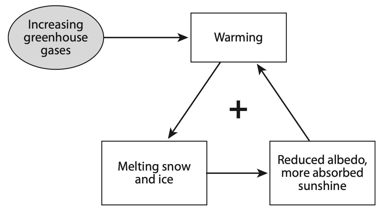
In a warmer climate, snow and ice cover are expected to decrease globally. The dependence of snow and ice cover on surface temperature is the first essential part of the snow and ice albedo feedback. A second essential part is that snow and ice absorb less solar radiation than the darker surfaces that they cover up. When dark soil or rock emerges from beneath white snow or a retreating glacier, or when the dark ocean emerges from beneath the white, sometimes snow-covered sea ice, more solar radiation is absorbed by the newly darkened surface. We therefore expect the albedo to decrease as the surface temperature increases. The reduced albedo leads to an increase in the absorption of solar radiation. The added solar energy causes warming, which, in turn, can cause even more melting. This is a ‘positive feedback loop’, as depicted below.

⊕Randall, Atmosphere, Clouds, and Climate, (2011).

The positive snow and ice albedo feedback can amplify a cooling, as well as a warming. If the climate cools, the resulting increased snow and ice cover reflects more sunlight back to space, and the cooling is amplified. Note that both positive and negative feedbacks can cause either warming or cooling; their role is to amplify or damp a given temperature change.

The Water Vapor Feedback

The water vapor feedback is the most important atmospheric feedback in the climate system. Its existence was recognized over a century ago by Svante Arrhenius in the 1890s, though it took until the late 1960s and the first computer-based climate modeling work to begin to understand its full significance.

The water vapor feedback is based on the principle that you can evaporate exponentially more water vapor into air as you increase the temperature. This is illustrated below, which is a plot of the ‘saturation vapor pressure of water’ as a function of temperature.

⊕Saturation vapor pressure, \(e^*\), as a function of temperature and in units of hectopascals or hPa. Air in the real world can have less or sometimes slightly more water vapor than this, but if the water vapor concentration gets too much higher than this curve, the water will condense out into water droplets or snow. Randall, Atmosphere, Clouds, and Climate, (2011).

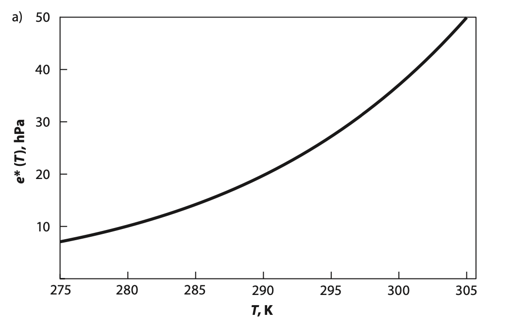
At the Earth’s globally averaged surface temperature of 288 K, the saturation vapor pressure increases by about 7% for a 1 K warming. Therefore the water vapor content of the atmosphere will increase by about 7% per K as the climate warms.Randall, Atmosphere, Clouds, and Climate, (2011). Because water vapor is a powerful greenhouse gas, that is, it strongly absorbs and emits infrared radiation, an increase in the atmospheric water vapor content causes an increase in the downwelling infrared radiation at the Earth’s surface. This further increases the warming and thus the initial perturbation is amplified. So the water vapor feedback is a positive feedback.

Surface evaporation can moisten a deep layer of air only if a mechanism exists to carry water vapor upward away from the surface. Turbulence of air currents near the surface helps, but it isn’t enough to bring water vapor higher than about 1 km. Further lifting of moisture is necessary if the total moisture content of the atmosphere is to increase by very much. The most important mechanism for such further lifting is cumulus convection (see below).Randall, Atmosphere, Clouds, and Climate, (2011). For this reason, convective clouds play an essential role in the water vapor feedback.

⊕A picture of small and large cumulus clouds, formed by convection or rapidly rising moist air. The air around the cloud towers is slowly sinking. Some of the larger towers have flat cloud layers near their tops. These are regions where the air has stopped rising and is flowing out to the sides. Randall, Atmosphere, Clouds, and Climate, (2011).

The mass of water vapor in the atmosphere exceeds the mass of carbon dioxide by about a factor of 4, and water vapor contributes more to the downward infrared at the Earth’s surface than \(\text{CO}_2\) does. Despite this, \(\text{CO}_2\) controls the greenhouse effect while water vapor plays a subservient role. Why is that? It’s because water vapor is condensible and can be removed from the atmosphere by precipitation, whereas \(\text{CO}_2\) does not condense under conditions found in the Earth’s atmosphere and can only be removed on very long timescales by rock weathering via the Urey reaction.

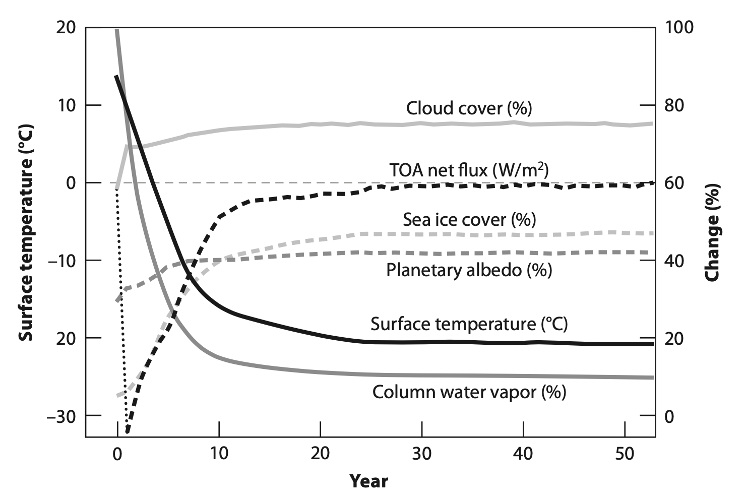
Lacis et al. (2010) illustrated the primary role of \(\text{CO}_2\) through a clever and simple experiment with a climate model. When run with realistic present-day \(\text{CO}_2\) concentrations, the model produces a realistic simulation of today’s observed climate. In the experiment, Lacis and colleagues removed all of the \(\text{CO}_2\) from the atmosphere. The results were spectacular. As we can see in the figure below, the surface temperature began to fall immediately as a direct result of the absence of \(\text{CO}_2\). This led to a reduction in the water vapor content of the atmosphere and additional cooling through the water vapor feedback. The positive snow and ice albedo feedback also reinforced the cooling (albedo increases over time). Within 10 simulated years, the Earth became almost completely covered in ice and had an atmosphere with very little water vapor.

⊕Time evolution of global surface temperature, top-of-the-atmosphere (TOA) net radiation, column water vapor, planetary albedo, sea ice cover, and cloud cover, after the zeroing out of the \(\text{CO}_2\). The initial conditions are for a preindustrial atmosphere. Surface temperature and top-of-the-atmosphere net radiation use the left-hand scale. Lacis et al., Atmospheric \(\text{CO}_2\): Principal control knob governing Earth’s Temperature, (2010).

Suppose that we ran a ‘mirror-image’ experiment, in which the \(\text{CO}_2\) concentration was realistic but the water vapor content of the atmosphere was set to zero at the beginning of the simulation. There would be a brief cooling but evaporation from the oceans would restore a realistic water vapor distribution within a few simulated weeks, and the simulated climate would stay close to what we observe today.Randall, Atmosphere, Clouds, and Climate, (2011).

An extreme version of the water vapor feedback, called a ‘runaway greenhouse’, likely occurred on Venus.Ingersoll, Planetary Climates, (2013). Venus is similarly sized compared to the Earth and very likely began its existence with a similar amount of water as the Earth. But Venus’ curse was that it was too close to the Sun, receiving significantly more solar radiation than Earth (in its early existence it would have received about 1/3 more than what Earth currently receivesCatling and Kasting, Atmospheric Evolution on Inhabited and Lifeless Worlds, (2017).). The extra solar radiation evaporated Venus’ oceans into its atmosphere, giving it a hot, moist, and dense water vapor atmosphere. This would have increased the surface temperature so much that no life could survive. Water vapor that was high in Venus’ atmosphere could also be blown apart by high energy photons, allowing the hydrogen to escape to space. The oxygen from the water vapor remnants would then combine with iron molecules at the surface so that eventually the hot Venus also lost its water.

While global warming will result in many negative outcomes, a runaway greenhouse is the only known mechanism by which global warming, in its severest form, could directly cause a collapse of global civilization or the extinction of humanity.⊕For more discussion of the existential risk posed by global warming, in the context of all other known existential risks, see: Ord, The Precipice: Existential Risk and the Future of Humanity, (2020). The best current estimate is that there is an approximately 1 in 1000 chance of the Earth crossing a point of no return in the next 100 years or so and eventually going into a runaway greenhouse state (or a practical equivalent known as a ‘moist greenhouse’ state where Earth is too hot to sustain life but not hot enough for the oceans to boil away into the atmosphere). Under this worst-case scenario, the climate system would need to be particularly sensitive to radiative forcing, humans would need to burn nearly all the available fossil fuels, and nearly all of the land carbon in peat deposits and ocean carbon in methane hydrates would need to be emitted by the warming Earth (recall Chapter 5). This 1 in 1000 chance is comparable to the estimated risk of global nuclear war in the next 100 years but more likely than the estimated risk of a supervolcano eruption (1 in 10,000) or a massive asteroid impact (1 in 1,000,000) occurring in the next 100 years. So in the unlikely event that we manage to bring about our own extinction due to global warming, it will be through the water vapor feedback.

The Lapse-Rate Feedback

Recall from Chapter 2 that the troposphere gets cooler with height. The rate that temperature decreases with altitude is called the atmospheric ‘lapse rate’. This can be described according to the equation, \(\Gamma = - \frac{dT}{dz} \), where \(T\) is the temperature and \(z\) the altitude or height. The negative sign convention gives a positive number for \(\Gamma\) in the troposphere. The global average lapse rate on Earth is about 6.5 K/km.

As the atmosphere warms there are basically three different ways that the lapse rate could change in the troposphere, as shown in the figure below, which shows shifts relative to a typical tropical lapse rate (black line). There could be a uniform warming shift (blue line), the lower part of the troposphere could warm more than the upper part (purple line), or the upper part of the troposphere could warm more than the lower part (orange line).

⊕

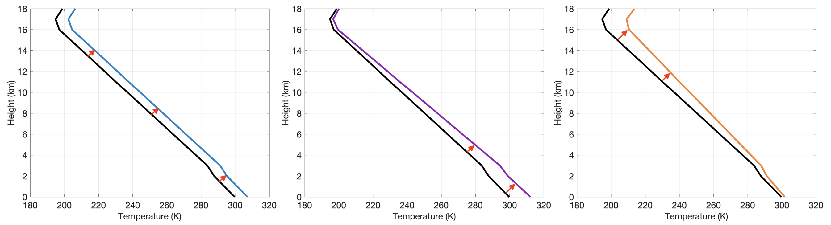
If the warming is uniform through the troposphere, with a lapse rate that does not change, then there is no strong lapse-rate feedback. But if the lapse rate changes, then there will be some interesting effects. Infrared photons that are emitted nearer to the surface have a harder time escaping to space because they are more likely to be absorbed somewhere in the atmosphere as they try to travel out to space. So a preferential warming of the surface, as in the purple line, ends up trapping more photons near the surface, which leads to more surface warming—a positive feedback. But if there’s preferential warming in the upper troposphere, as in the orange line, photons have an easier time escaping to space, meaning that a warming would lead to more efficient cooling—a negative feedback.

So under global warming, which of these occur? The answer is actually all three: different regions on Earth have different lapse rate responses (see figure below). But on a global average, the lapse rate response in the tropics ends up being much stronger than anywhere else, leading to an average preferential warming with height (a decreased lapse-rate), and thus a negative feedback.

⊕The spatial pattern of the lapse rate feedback (labeled as \(\lambda(r)\) in the plot) in the CCSM4 global climate model. Armour et al., Time-Varying Climate Sensitivity from Regional Feedbacks, (2013).

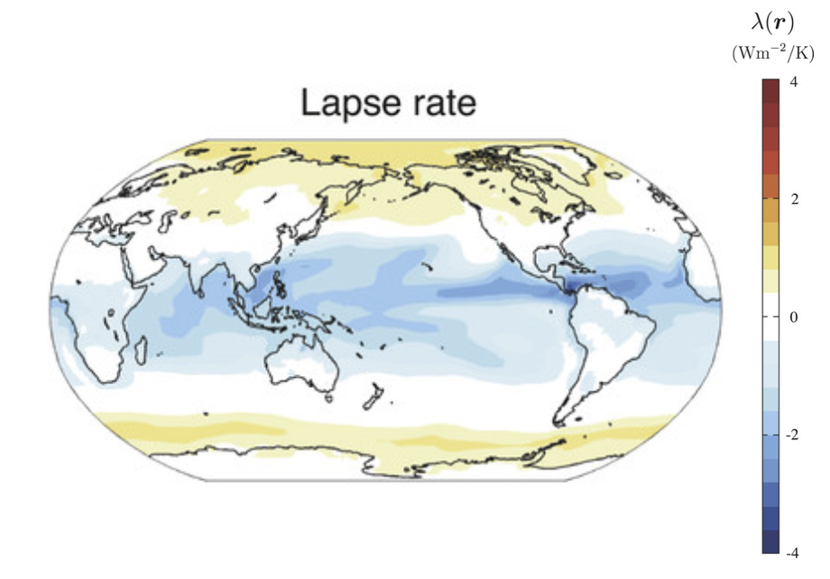
Why do the tropics have a preferential warming with height? The tropics have a lot of rising moist air or moist convection, much more than anywhere else on Earth. And when the air rises and cools, eventually water will begin to condense out of the gas phase and into the liquid phase, thus forming clouds. But the transition from gas to liquid converts some potential energy into kinetic energy, usually called ‘latent heating’.Bohren and Albrecht, Atmospheric Thermodynamics, (2023). (Just the opposite process happens when you boil water: you have to add energy to transition the water from liquid to gas.) So the atmosphere gets a boost of kinetic energy, thus warming it, as the moist air rises and condenses into clouds. In a warmer world, you can evaporate more water into the air, so there will be more potential energy available. This leads to preferential warming with height and thus the tropics have a negative lapse rate feedback.

Cloud Feedbacks

Cloud feedbacks are infamous. Their potential importance has been recognized at least since the 1970s. For decades, they have been highlighted as a major source of uncertainty in predictions of future climate change. Why is the problem taking so long to solve?

Although cloud processes are among the most important for climate, they are also among the most difficult to understand and predict. Cloud processes can be grouped into five categories, all of which are important for the climate system:Randall, Atmosphere, Clouds, and Climate, (2011).

1. Cloud microphysical processes, involving cloud drops, ice crystals, and aerosols, with scales on the order of microns
2. Cloud dynamical processes associated with the motion of the air in cumulus clouds, with scales on the order of a few kilometers
3. Cloud radiative processes, involving the flows of both solar and terrestrial radiation through the cloud field
4. Cloud turbulence processes, which include near-surface turbulence, the entrainment of environmental air into the clouds, and the formation of small clouds
5. Cloud chemical processes, which, among other things, are important for the annual formation of the ozone hole through the destruction of ozone in polar stratospheric clouds

These various processes interact with each other on space scales of meters to kilometers and time scales of a few minutes. These processes also interact with larger-scale weather systems, up to the size of the Earth itself. Clouds are therefore difficult to understand and predict because of these complexities.

While there are many different kinds of cloud feedbacks, the ones with the largest radiative impacts are most important. The impacts can affect the incoming solar radiation and/or the outgoing infrared radiation.

Nearly all cloud types behave like blackbodies because they are composed of liquid water droplets or ice crystals. We learned in Chapter 3 that water vapor can absorb radiation in continuum sections of the radiation distribution instead of in lines or bands like most other gases. It turns out that water droplets and ice crystals are even better blackbodies than gaseous water vapor. Clouds are therefore good at absorbing and emitting infrared radiation.

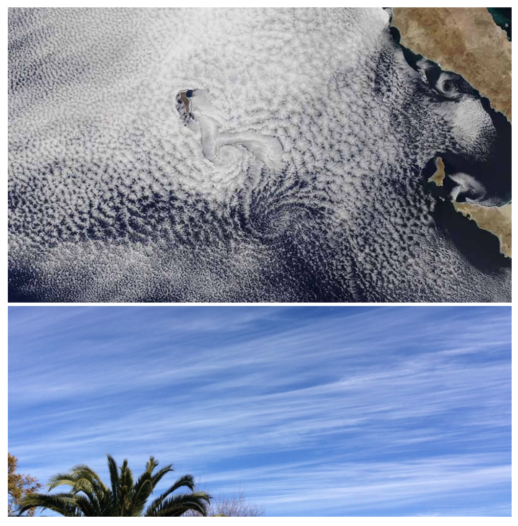
How clouds interact with solar radiation is more complicated than infrared radiation. Solar radiation can be reflected (albedo is the fraction that is reflected), it can be absorbed, or it can pass through the cloud (called transmission or opacity); each of these depends on the cloud thickness, the amount of liquid water or ice in the cloud, and the size of the cloud’s water droplets or ice crystals. For example, marine stratocumulus clouds often have high albedos and overlay the low albedo ocean, see below; like the ice-albedo feedback, this property makes changes in marine stratocumulus clouds particularly important. In contrast to these, high cirrus clouds have a low opacity and let a lot of solar radiation through, see below.

⊕Top: Marine stratocumulus clouds off the western coast of Mexico, NASA. Bottom: Cirrus clouds over Adelaide Australia, Joseph Nicholls.

How will clouds change with global warming? The schematic below shows the radiatively important changes, along with their associated feedbacks (positive in red, negative in blue, or uncertain in purple), illustrated from the tropics to the polar regions.

⊕Different cloud changes and their associated feedbacks (\(+f,\,-f,\,\pm f\)) under global warming. The schematic is adapted from IPCC, AR6, Chapter 7.

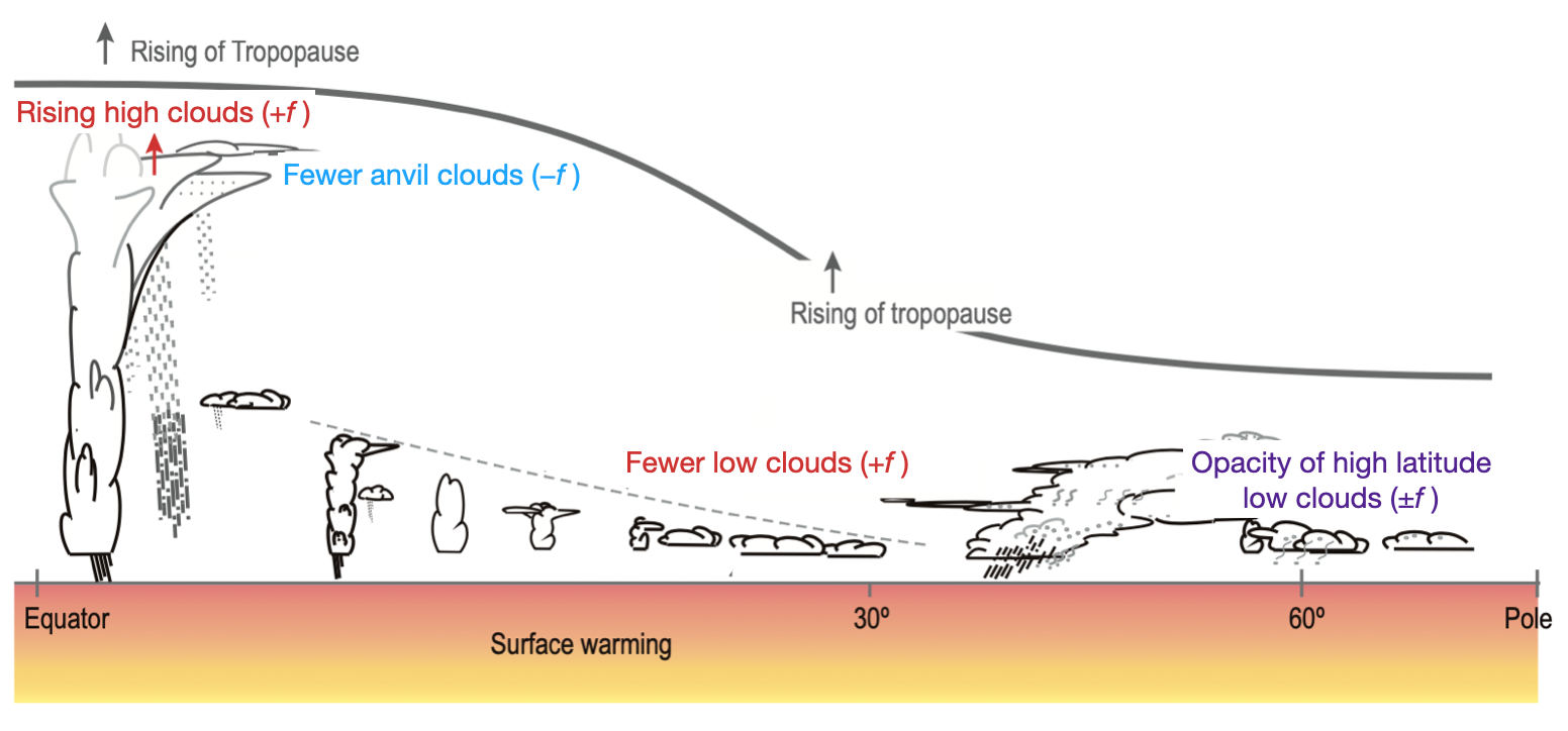
Let’s walk through each of these changes. The tropopause rises and along with that high tropical cumulus clouds also rise. But there’s a curious feature of these clouds. Even though they get taller, the tops remain approximately the same temperature, about 200 K. This means that the outgoing infrared radiation from these clouds can’t change even though the surface is warming.Zelinka and Hartmann, Why is longwave cloud feedback positive?, (2010). If they can’t emit more radiation to space, that radiation will stay near the surface and lead to further warming, which is a positive feedback.

Next on the diagram we see that there will be fewer ‘anvil’ clouds. You can see examples of such clouds in the picture of cumulus clouds in the ‘Water Vapor Feedback’ section. The anvil clouds have high albedos, so fewer of them could lead to more absorbed solar radiation at the surface. But they are also big blackbodies in the sky that increase the amount of infrared radiation re-emitted back down to the surface; it turns out that this infrared effect is larger than the albedo effect.Sherwood, et al., An Assessment of Earth’s Climate Sensitivity Using Multiple Lines of Evidence, (2020). So on balance, fewer anvil clouds leads to a net cooling, a negative feedback.

Fewer low clouds, especially fewer marine stratocumulus clouds, means that more solar radiation will hit the ocean or Earth surface instead of being reflected back to space. So a warming that produces fewer low clouds will increase the surface warming, a positive feedback.

Lastly, it’s currently unclear whether low clouds in the high latitudes will change their opacity. If they allow more light through, they would be a positive feedback; if they allow less light through, they would be a negative feedback. There are reasons to think it could go either way by a significant amount and not enough conclusive data and model evidence currently exists.Sherwood, et al., An Assessment of Earth’s Climate Sensitivity Using Multiple Lines of Evidence, (2020).

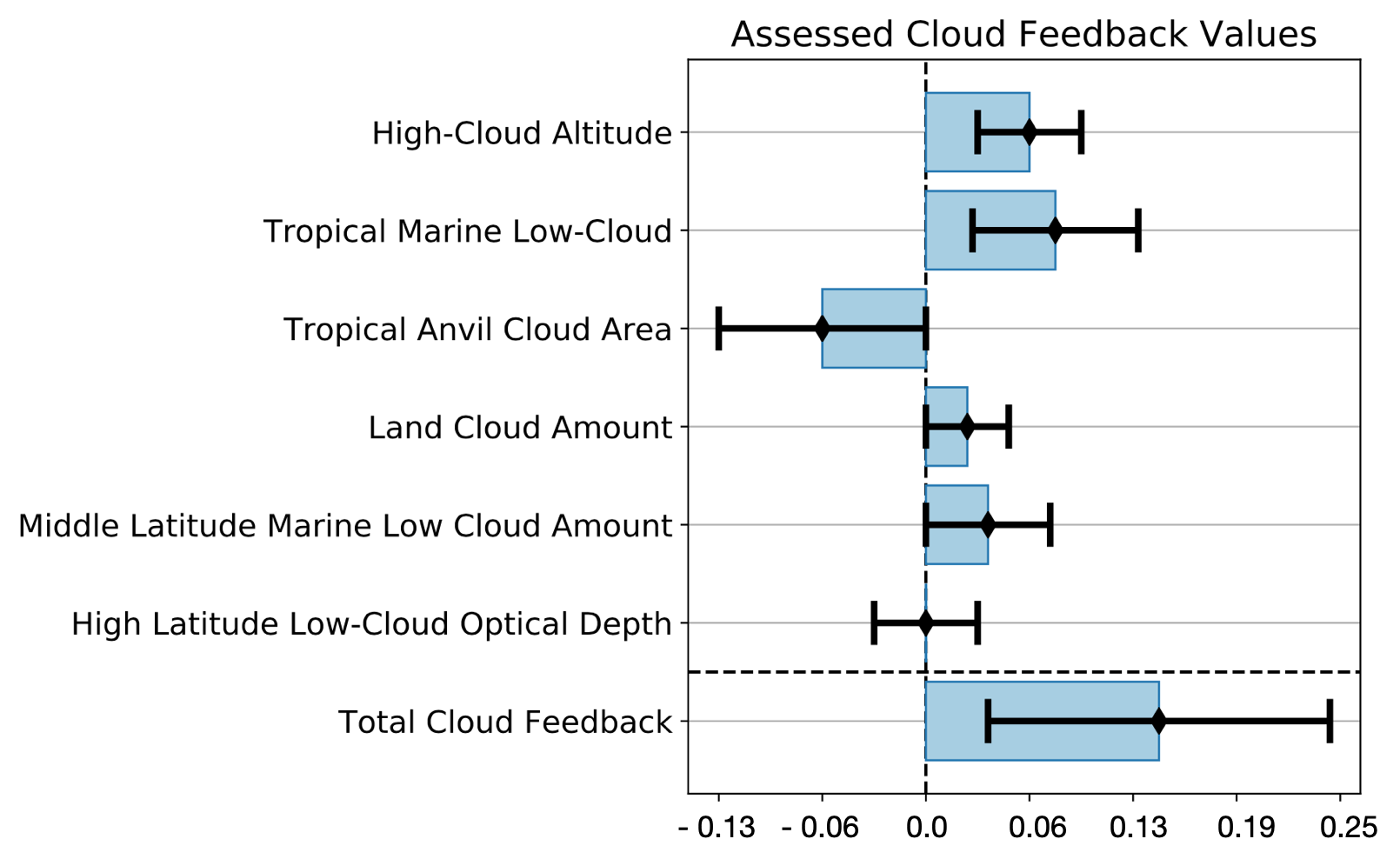
The figure below summarizes the numeric values of all these categories of feedbacks (blue bars) along with their uncertainties (black error bounds). Combined, they amount to a positive feedback, though the uncertainties are fairly large. Studying and trying to improve our understanding of cloud feedbacks is a big challenge and one of the most active areas of research in climate science.

⊕Sherwood, et al., An Assessment of Earth’s Climate Sensitivity Using Multiple Lines of Evidence, (2020).

Climate Sensitivity

In this chapter we have discussed the four most important climate feedbacks: albedo, water vapor, lapse rate, and cloud. While there are other feedbacks, they are small compared to these four and don’t contribute significantly to the overall feedback of the climate system. With both positive and negative feedback processes in the climate system, it’s not clear at first glance what the overall response to global warming will be. For example, we saw that tropical convection could lead to both a negative lapse-rate feedback and also a positive high-cloud altitude feedback. How do all of these combine and which are most important?

To explore this, let’s return to the equations from the first part of this chapter. We found that a change in temperature due to a change in radiative forcing, accounting for feedbacks, could be described by the following equation, \[\Delta T = \frac{\lambda \Delta R}{1-f} \; .\] We computed that a no-atmosphere planet would have a climate sensitivity parameter of \(\lambda = 0.27\,\text{m}^2\text{K}/\text{W}\). For Earth with a realistic atmosphere, but with feedbacks turned off, it turns out that \(\lambda = 0.31\,\text{m}^2\text{K}/\text{W}\). We know that the feedbacks \(f\) are going to have to be calculated based on what the climate system is like. Though we should note that for a stable climate system \(-\infty < f < 1\). But what value should we use for \(\Delta R\), the change in radiative forcing? There have been many different radiative forcings that the Earth has experienced and because we don’t know for sure how humans will act in the future, we don’t know what the cumulative radiative forcing will be due to global warming once it is all done. A useful experimental framework that makes this easier and more unified is to use a \(\Delta R\) that represents a doubling of \(\text{CO}_2\). It turns out that the total radiative forcing from any doubling of \(\text{CO}_2\) in Earth’s atmosphere is approximately the same, no matter the starting value (e.g., \(\Delta R\) is the same going from 10 ppm to 20 ppm or 400 ppm to 800 ppm).If you are reading this as part of my course, you may recall this fact from a previous assignment! In a realistic Earth atmosphere this works out to be \(\Delta R_{2xCO2} = 4.0\, \text{W}/\text{m}^2\).

The annual- and global-mean surface air temperature response to a doubling of \(\text{CO}_2\) is known as the ‘climate sensitivity’. Mathematically it can be written as, \[\Delta T_{2xCO2} = \frac{\lambda \Delta R_{2xCO2}}{1-f} \; .\] Climate sensitivity is a central topic in the science of global warming. In fact many debates about global warming are often debates about the numeric value of Earth’s climate sensitivity because it is the theoretical concept that explains how much warming we can expect to see.

If there were no feedbacks, what would Earth’s climate sensitivity be? With \(f = 0\) and using the values of \(\Delta R_{2xCO2}\) and \(\lambda\) above, we have that \(\Delta T_{2xCO2} = 1.2\, \text{K}\). What about if we add in the ice albedo feedback, \(f_a\)? The current best estimateSherwood, et al., An Assessment of Earth’s Climate Sensitivity Using Multiple Lines of Evidence, (2020). of \(f_a\) is 0.09, so that works out to \(\Delta T_{2xCO2} = 1.4\, \text{K}\). So the albedo feedback only increases the temperature by about 0.2 K, which isn’t much.

What if we put them all together? The total feedback factor is equal to the sum of the albedo, water vapor, lapse rate, and cloud feedback factors, so \[f=f_a+f_w+f_\Gamma+f_c=0.59\;,\] a value based on recent estimates.Sherwood, et al., An Assessment of Earth’s Climate Sensitivity Using Multiple Lines of Evidence, (2020). The climate sensitivity including all these feedbacks comes out to \(\Delta T_{2xCO2} = 3.0\, \text{K}\). So a doubling of \(\text{CO}_2\) is estimated to result in about 3 degrees of global-mean warming. If we compare this value with the no-feedbacks case, we see that feedbacks amplify the warming and contribute about 2 degrees for a \(\text{CO}_2\) doubling. This is a big difference. The global warming we’ve experienced thus far since the 1800s is about 1.3 K. If there were no climate feedbacks, keeping global warming in check would be much easier.

A very important issue we’ve so far neglected in this discussion about climate sensitivity is the uncertainties involved. The calculations we’ve made here are for the average estimates of \(\Delta R_{2xCO2}\), \(\lambda\), and \(f\). If you include the uncertainties in each, climate sensitivity is not a single value but actually a distribution of values. And then if you include or exclude certain kinds of information, you can even produce different distributions to further sample the range of uncertainty. One ambitious studySherwood, et al., An Assessment of Earth’s Climate Sensitivity Using Multiple Lines of Evidence, (2020). set out to include as much information as reasonably possible to estimate climate sensitivity, see below. The most important distribution to look at is the black ‘Baseline PDF’ plotted below.

⊕Several estimates of climate sensitivity based on climate model evidence, observational evidence, paleoclimate evidence, and expert evaluations (a Bayesian combination of all these). The thick black line shows the full climate sensitivity distribution, with colored lines showing how the black distribution would change if different kinds of data were excluded. Circles on the distributions indicate 17th and 83rd percentile values. The lines at the top show the central 66% range of the Baseline PDF (gray), all the plotted distributions and titled ‘Robustly’ (magenta), and from the AR5 report of the IPCC (cyan). Adapted from: Sherwood, et al., An Assessment of Earth’s Climate Sensitivity Using Multiple Lines of Evidence, (2020).

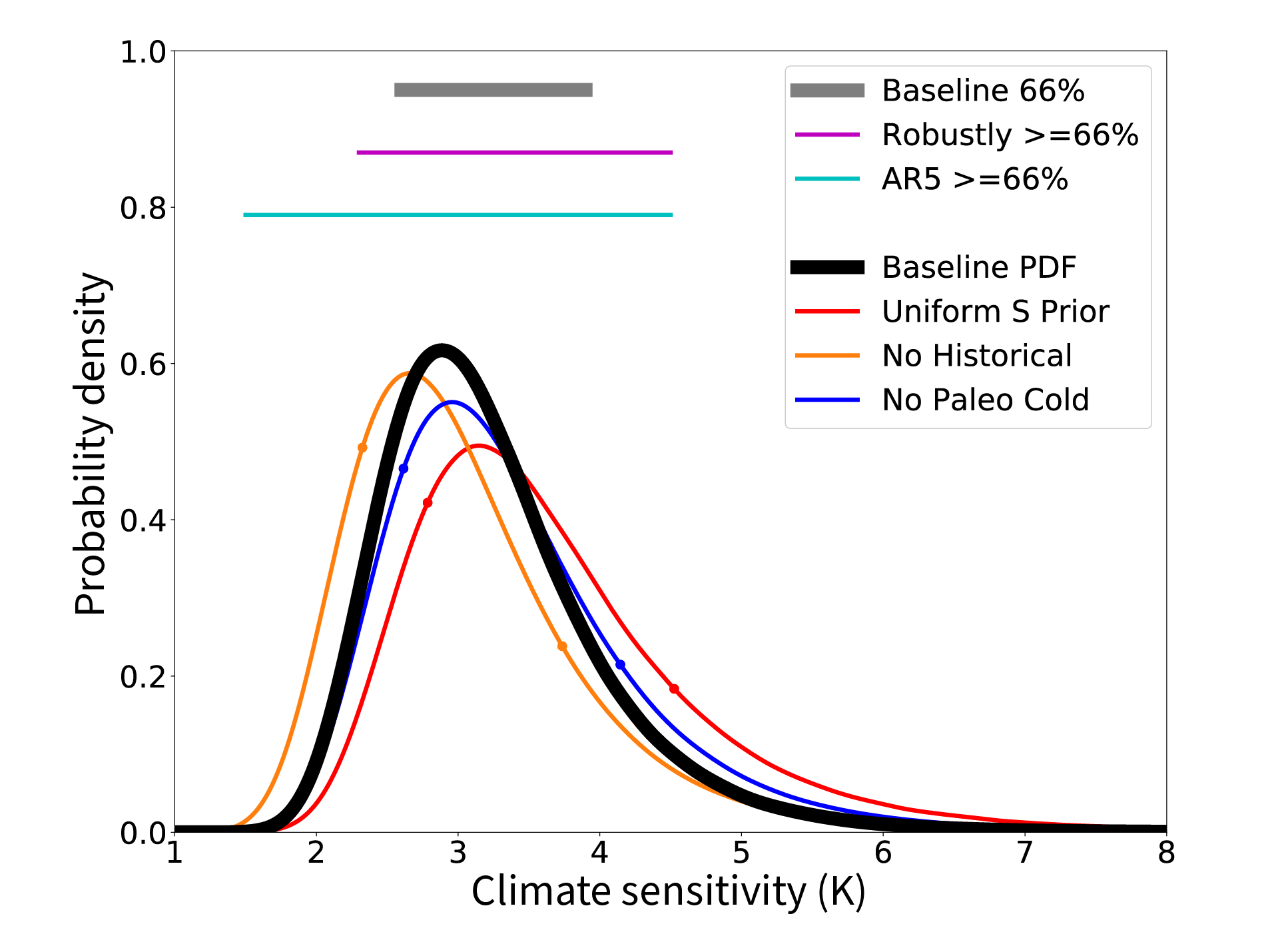
You can see that the most likely value of climate sensitivity is about 3 K. But the distribution spans a fairly wide range with the 5th to 95th percentile range being 2.3-4.7 K. Smaller values indicate a climate that is less sensitive to radiative forcing while higher values indicate a climate that is more sensitive. Note also that the distributions are ‘fat tail’ distributions: high values of climate sensitivity cannot be ruled out until about 7 K.

\(\Uparrow\) To the top

\(\Rightarrow\) Next chapter

\(\Leftarrow\) Table of contents