Radiative-Convective Models
Simple Climate Models
The climate models that we have learned about so far are of the simplest kind: energy balance models. In Chapter 3 we learned about a model that had only a single layer of atmosphere in it, reproduced below.
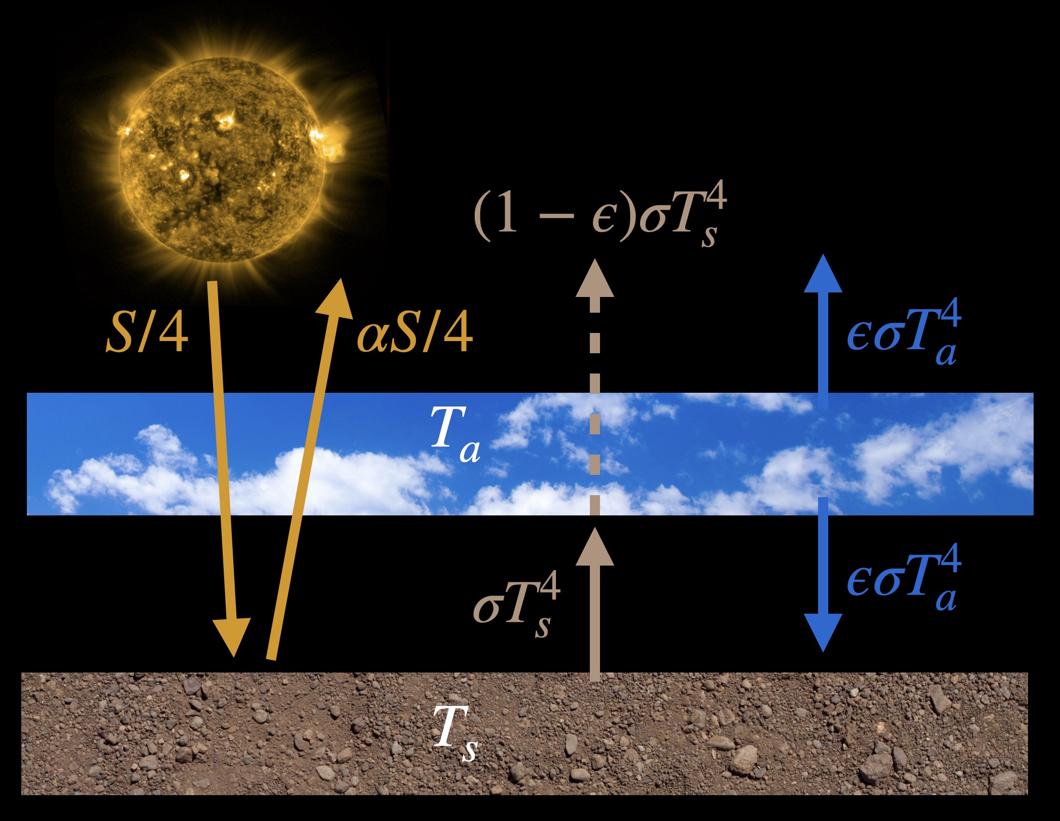
Even though we could get a lot of insight about the climate of Earth from this model, it isn’t suited to asking all sorts of questions we might like to answer. The model doesn’t have clouds, it doesn’t rain, it doesn’t have an ocean or land plants. The atmosphere doesn’t move around and it doesn’t model radiation in a very sophisticated way. There are a lot of things it doesn’t have. Because it’s missing all these kinds of parts we can’t even properly ask questions like: How much does temperature change by doubling CO2? Or how will global warming unfold?
The next level up in climate model complexity is what’s known as a one-dimensional (1-D) vertical column model of the atmosphere. To visualize these models, imagine taking a 1 meter-squared column of atmosphere from the surface to the top and making a mathematical model of that with about 20 or so layers. The simplest versions of these models assume that that column of air is even isolated from any air around it, sort of like if it were placed inside a very tall tube.
1-D column models were first developed in the 1960s and some fundamental climate science work was done using these models. In fact, the primary scientist who developed them, Syukuro Manabe, won the Nobel Prize in Physics in 2021, for his work using 1-D atmospheric column models, and later 3-D global climate models. This was the first time that a climate scientist was ever awarded the Nobel Prize in Physics. Another climate scientist, Klaus Hasselmann, was co-awarded the Nobel this same year for his fundamental work on modeling the ocean. Such 1-D models are sufficiently realistic that you can ask questions like what the climate sensitivity is, but they are also simple enough that they aren’t hard to understand. So before we get to learning about the complex, 3-D atmosphere-ocean-land climate models in the next chapter, we’ll start here with the simpler 1-D models.
Our journey into the world of 1-D models will consist of understanding the key results from experiments that Manabe and colleagues performed and published in the 1960s. These have been called ‘the most influential climate science papers of all time’.
Radiative-Convective Equilibrium
Manabe and colleagues at the ‘Geophysical Fluid Dynamical Laboratory’ of what was then the United States Weather Bureau, developed the first realistic 1-D atmospheric column model. It had 18 layers in it. They called their model a ‘radiative-convective’ model because it could transfer energy up and down by ‘radiating’ it (like in our energy balance model) and by ‘convecting’ or moving air up and down. The model also included clouds in a basic way. It calculated the solar and infrared radiation exchanges using a method that accounted for the radiative characteristics of all the major greenhouse gases; the model could therefore account for changes in different gas concentrations.
In the model, convection was represented by a procedure called ‘convective adjustment’. Convection normally happens in the atmosphere when the air is unstable, like when high energy air is below low energy air. Just as a hot air balloon will rise when the air inside it is heated, so will a chunk of air rise up if it has higher energy than the air around it. So in Manabe's model, when the lapse rate became physically unstable, the lapse rate was ‘adjusted’ or changed back to a stable lapse rate of 6.5°C/km (which is the global average lapse rate value). This adjustment was performed such that the total energy of the column was conserved.
Manabe initialized the model with initial conditions reflective of the average observed concentrations of greenhouse gases, but with an atmosphere that had the same temperature from top to bottom. The model was solved numerically in small time steps (similar to how weather forecast models are run today) and the vertical temperature profile adjusted over time until it reached a steady ‘equilibrium’ state. The figure below shows how the vertical temperature profile adjusted from two different hot and cold conditions over time. The temperature converges over time until it gets to the stable equilibrium temperature profile shown by the thick solid black line.
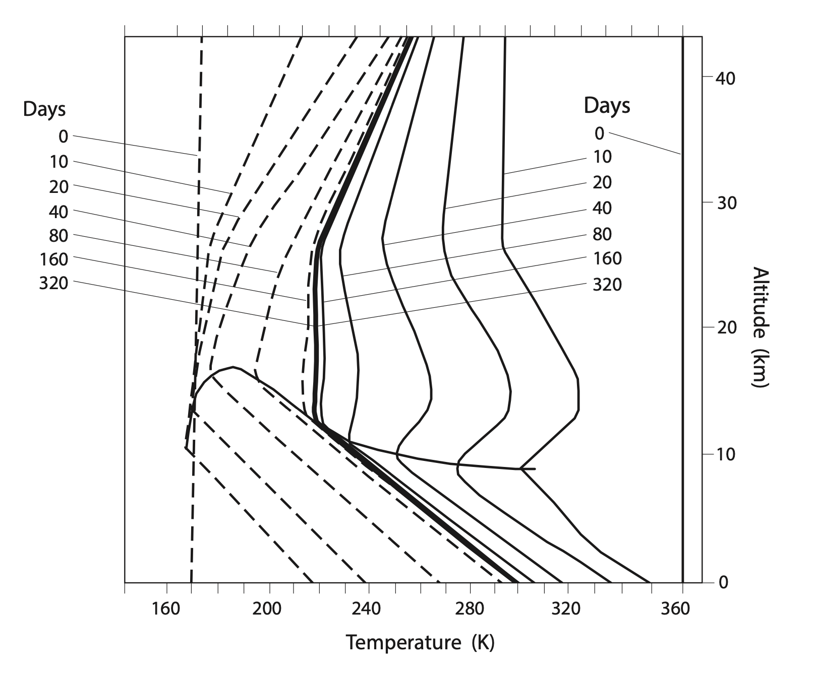
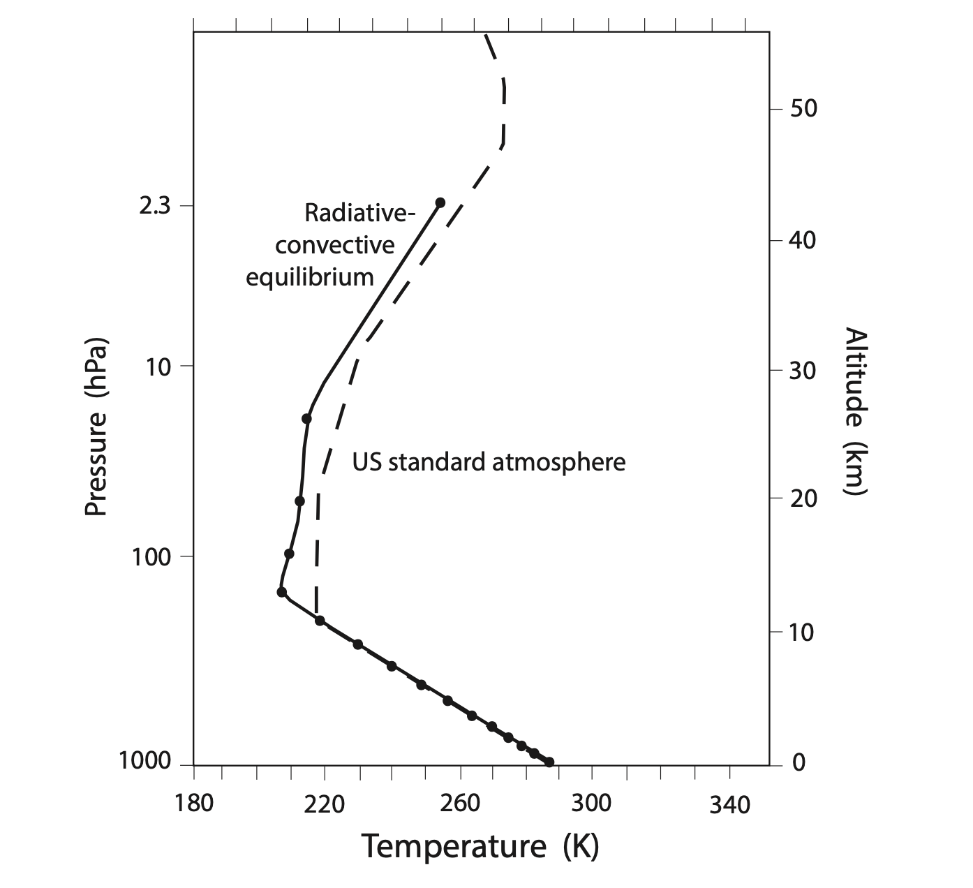
This thick black line shows a troposphere that cools with height, following the 6.5°C/km lapse rate, and a stratosphere that warms with height. The general shape of the profile compares well with the observed ‘US standard atmosphere’, both plotted together below.
Previous models of the atmosphere were basically just energy balance models (some with many layers) that could only radiate energy. So how does the addition of convection change the temperature of the atmosphere? To explore this, Manabe ran an additional simulation that turned off the convection, so that energy balance could only happen through radiation. Results comparing the radiative-convective equilibrium with the radiative-only calculation are shown below.
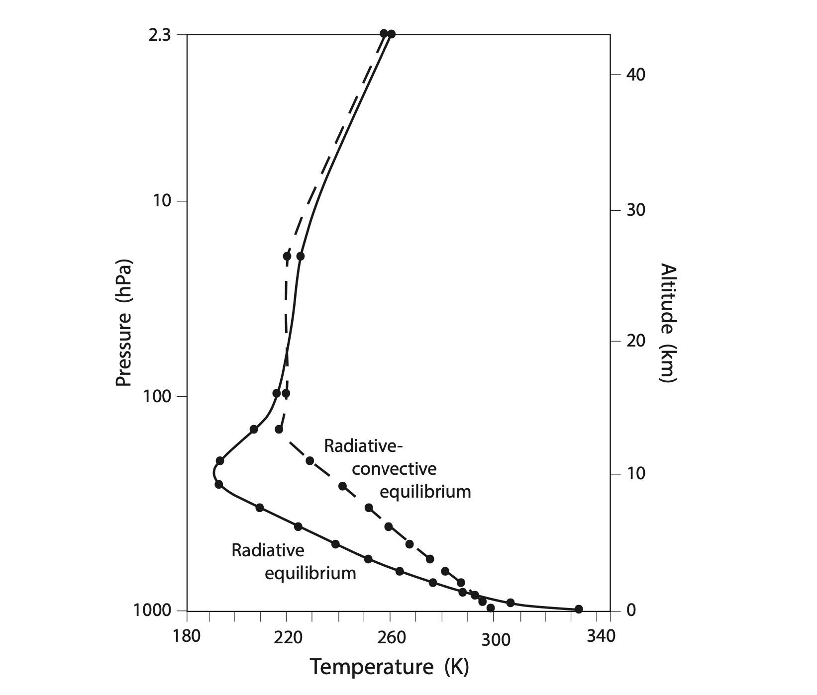
In this figure we can clearly see that convection has a big impact on the lapse rate and surface air temperature. Without convection, Earth’s surface air temperature would be about 333 K or 60°C, compared to 300 K or 27°C in the experiment with convection. Also, with no convection, the lapse rate would be about 14°C/km, much larger than the observed 6.5°C/km. Convection therefore evens out the troposphere’s temperature: it cools the surface and warms the upper troposphere.
The stratospheres aren’t very different from each other in these two experiments because there’s no convection in the stratosphere; the only way it can transport energy up and down is through radiation.
Heating and Cooling the Atmosphere
How is the atmosphere heated and cooled? And is radiation or convection more important for transporting energy? We can discover this by looking at how each of these processes heats or cools the atmosphere with height, shown below.
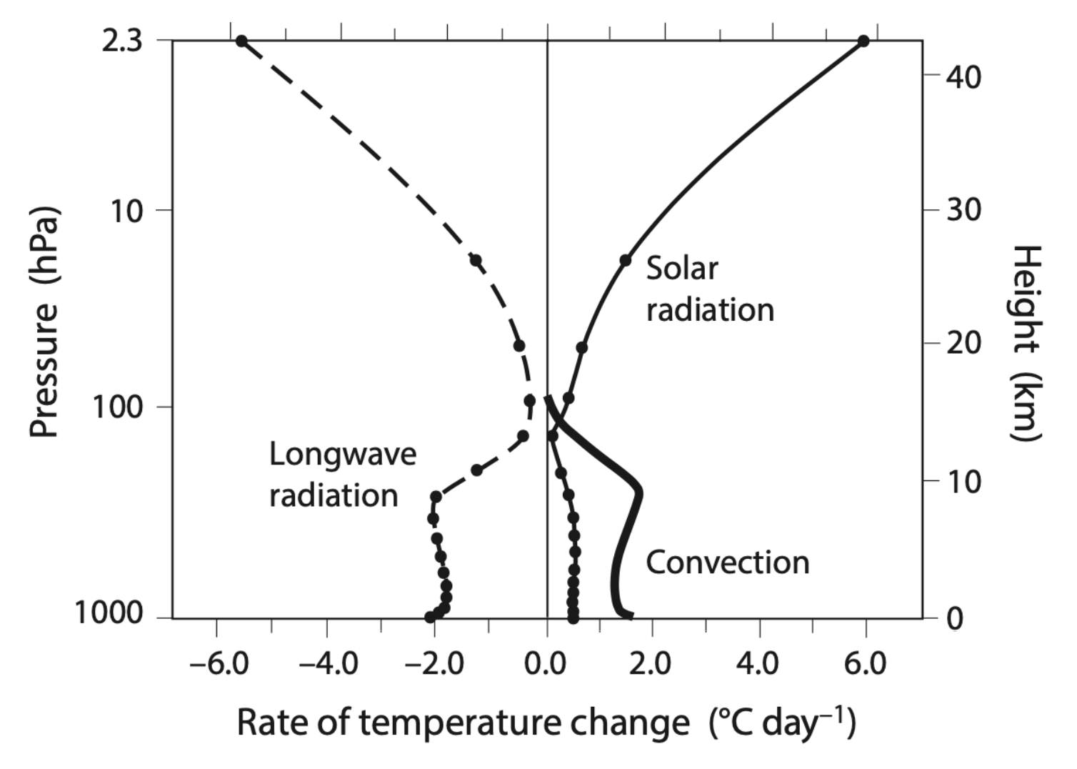
In this figure we can see that infrared radiation, called ‘Longwave radiation’, is what cools the atmosphere at all levels; note that longwave radiation does also heat parts of the atmosphere, but its cooling rate is larger than its heating rate when added together. What heats the atmosphere is solar radiation and also convection. Surprisingly, convection does more of the heating in the troposphere than solar radiation does; what it’s doing is transporting heat from the surface to the middle and upper portions of the troposphere. We can see, from this figure combined with the previous figure, that convection is a more efficient heat transport mechanism in the atmosphere than radiation.
What gases in the atmosphere are doing the radiative cooling and heating? The figure below shows the heating and cooling contributions of each gas as a function of height.
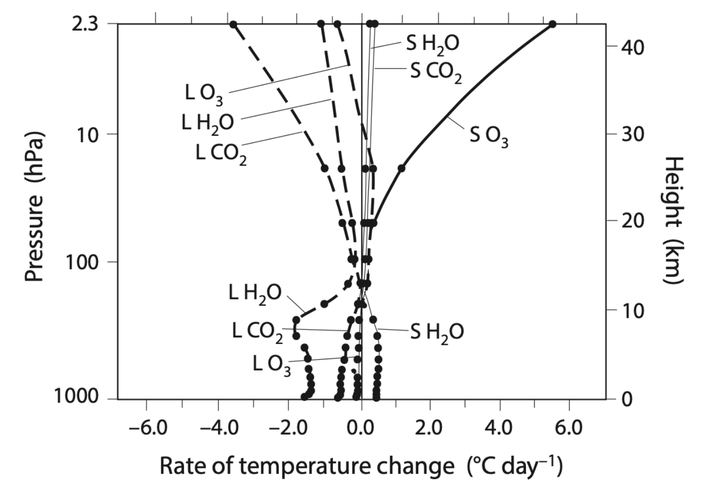
Let’s start by looking at the solar radiation heating side of the graph. At the top we see that solar radiation absorption by ozone, \(\text{O}_3\), is the reason we have a warm stratosphere (as we learned in Chapter 2). There are also small contributions to solar heating of the stratosphere from water vapor and carbon dioxide.
In the troposphere the only non-convective net heating is from water vapor absorbing solar radiation. Why doesn’t CO2 show up as heating the troposphere? It does heat the troposphere but only in the longwave and it also cools in the longwave too; if you add these together, the cooling impact has a larger magnitude than the warming impact and so the ‘L CO2’ line is shown to be negative. This might seem counter-intuitive, but keep in mind that what we are looking at here are the net rates of heating and cooling in the atmosphere due to radiation and not the magnitude of how hot the surface is. Specifically, the rates of temperature change are calculatedPeixoto and Oort, Physics of Climate, (1993). as \(\partial T/\partial t = 1/(c_p \rho) \partial F_{\text{net}}/\partial z\), where \(F_{\text{net}}\) is net radiation at a given level in the atmosphere; this is different than simply surface \(T\). The presence of greenhouse gases makes the surface warmer than it otherwise would have been without them. And if you increase the greenhouse gases, it warms the surface further. But when you look only at the rates of radiative heating and cooling in the atmosphere, CO2 provides a net longwave cooling of the atmosphere.
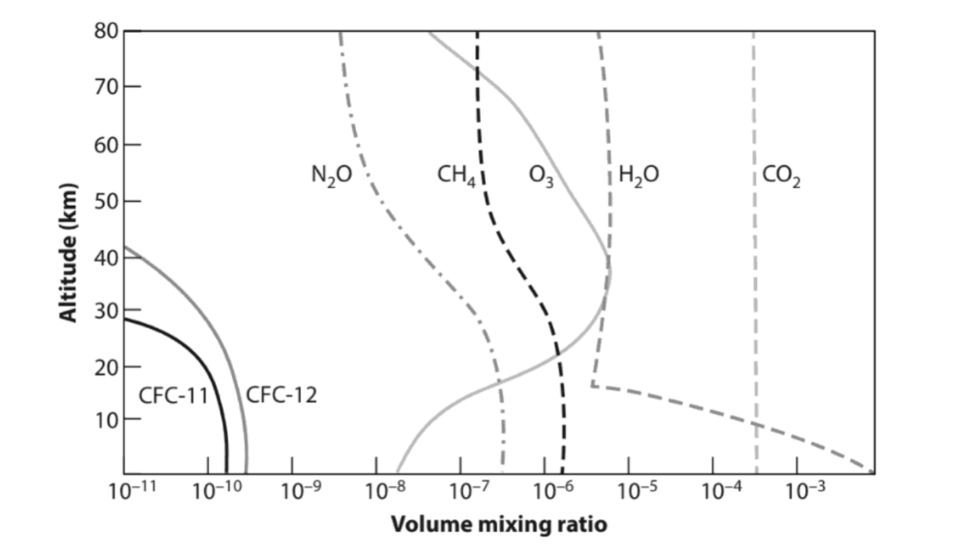
The left hand side of the graph above shows us which gases cool the atmosphere. In the stratosphere the largest one is CO2, followed by water vapor. But this is reversed in the troposphere, with water vapor doing the largest amount of cooling and CO2 in second place. This is because the vertical distributions of CO2 and water vapor are very different: CO2 is relatively consistent with height while water vapor is in large amounts only at the surface, see below.
Temperature Response to Doubling CO2
We learned in Chapter 1 that Svante Arrhenius was the first person to attempt a calculation of the effect of doubling CO2 in the atmosphere. But his data and methods were not really up to the challenge. It was therefore something of an accident that he got a climate sensitivity, 6°C, roughly consistent with current estimates. In order to calculate it properly one really needs good radiative absorption and emission data on atmospheric gases, a good mathematical model of the atmosphere, and a computer to run the calculations. Arrhenius didn’t have any of these. But Manabe and colleagues did, and they were the first to make a realistic calculation of what has come to be called Earth’s climate sensitivity.
Manabe used the same model as in his previous paper discussed above, to estimate the atmosphere’s response to doubling and halving CO2. The reference or control simulation used 300 ppm of CO2 (approximately the atmosphere’s value in the 1960s), and doubling and halving amounts of 600 ppm and 150 ppm. Just like the previous simulations they ran each of these until they reached an equilibrium state. The figure below shows the vertical profiles of temperature in radiative-convective equilibrium from these three experiments.
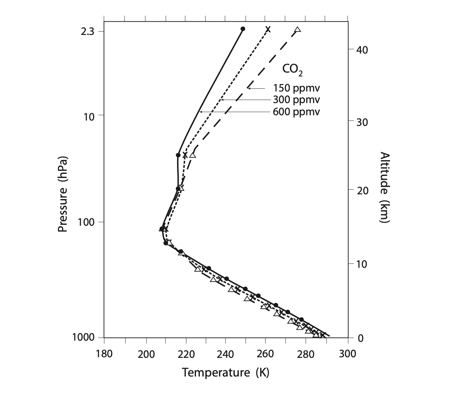
For the control simulation with a CO2 concentration of 300 ppm, surface air temperature is 288 K (~15°C), which is similar to the observed global mean surface temperature. In response to doubling CO2 to 600 ppm, the surface air temperature increased by 2.4°C. In response to halving CO2, surface air temperature decreased by 2.3°C. Note that unlike more recent calculations with more accurate models, the lapse rate in this model stays the same, at 6.5°C/km, instead of decreasing, on a global average, like we learned about in the last chapter. This is because of how the ‘convective adjustment’ was calculated in the model.
So Manabe calculated a climate sensitivity of about 2.4°C. This is fairly close to the current best estimate of 3.0°C, derived from far more sophisticated models.
You may have noticed from the figure above that as you increase CO2, the stratosphere actually cools, which is the opposite of the troposphere and the surface. We can explain this result by consulting the figure we saw before which shows the radiative heating and cooling effects of different gases:
We can see that the stratosphere is mostly heated by ozone’s absorption of solar radiation and cooled through the combined net longwave effect of CO2, ozone, and water vapor. So if CO2 is increased throughout the atmosphere, more CO2 in the stratosphere will lead to more cooling there.
\(\Uparrow\) To the top
\(\Rightarrow\) Next chapter
\(\Leftarrow\) Table of contents