Climate Variability from the Atmosphere and Ocean
Revised and adapted from ‘Climate and the Oceans’, Geoffrey Vallis (2011)
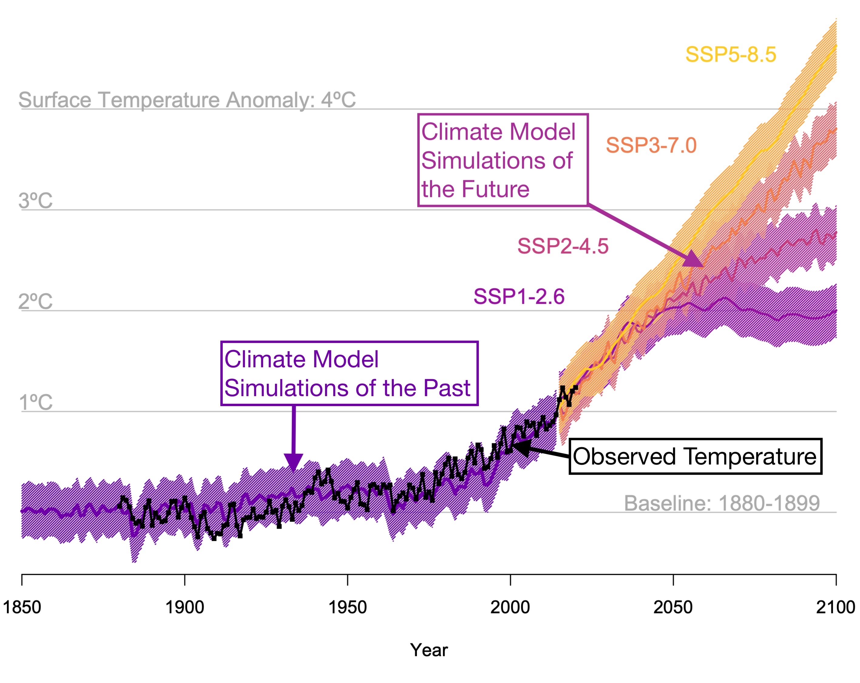
In this book’s motivating figure we see that the evolution of global mean temperature isn’t smooth but squiggles up and down. Why is this the case? It really has to do with the inherent timescales of the climate system and how they impact the global mean temperature. The first timescale we’ll look at is the weather timescale and how it is different from climate.
Weather and Climate
What is the difference between weather and climate? It is intuitively clear what the weather is—it is the day-to-day state of the atmosphere at some location, usually with reference to temperature, windiness, and precipitation. But when we speak of climate we wish to average out all these day-to-day fluctuations and refer to some kind of average of the weather. But what precisely? There is no ideal definition of climate, but the most common is that climate is the statistics of the weather—the mean, the standard deviation, and so forth. But do how we calculate the statistics—how do we take the mean, for example? And if climate is a time average of the weather, then how can climate have any temporal variability?
Although it is rather fanciful, it is useful to envision a thought experiment in which we take the ensemble average of the weather. Thus, we envision a large number of identical planet Earths, forced the same way, but each one started out in a slightly different way so that each has different weather. We could then unambiguously define the climate to be the average, along with other relevant statistical quantities like the variance, over the ensemble of planet Earths. If the forcing were to change, perhaps because the CO2 levels in the planets were to increase, then the climate of the ensemble would also change.
The problem with this definition is that it is not practical, there is no such ensemble in reality. However, we can try to take our average in such a way that it mimics the ensemble average as closely as possible, and this way of proceeding will be useful to the extent that the weather and climate have different time and space scales. We could then define climate as the average of the weather over a time period long enough so that weather fluctuations are averaged out but variability on longer timescales is still allowed. Weather typically varies on timescales of a few days to a few weeks, so that we might define climate as the average weather over time periods longer than a month. In practice, this time period is too short for many purposes because the monthly average temperature still fluctuates considerably, and a more common definition takes the climate to be the average (along with other statistical quantities) over a period of a few years, with the precise averaging period depending on what quantity is of interest. We might choose to take the average over a particular time of year—only over the winter months, for example, and so obtain a winter climatology. If we are interested in how climate varies across ice ages, then averaging over a period of centuries or even millennia might be appropriate, but if we are interested in whether climate changed over the course of the twentieth century, a much shorter period is obviously more appropriate.
The moral of the above discussion is that, although it is useful to think of the climate as some kind of average, there is no compact single definition of climate that is useful and appropriate for all purposes, and we are often better served by talking about the climate with reference to a particular timescale. Climate varies on more than one timescale—indeed, there is no timescale on which there is no climate variation.
Weekly Variability and the Weather
On daily and weekly timescales, the main mechanism that causes variations in the temperature and wind is simply the familiar weather. The mechanism that gives rise to weather resides in the atmosphere, and it is the consequence of a fluid instability called baroclinic instability. This instability can be thought of as a type of convective instability in which if a fluid is heated from below it expands, becomes lighter than its surroundings, and therefore rises or ‘convects’. Baroclinic instability has a similar origin, but it also involves the lateral motion of air, with a typical scale of up to a few thousand kilometers and a typical velocity of about 10 m/s. It takes a parcel of air moving at this speed a little more than a day to travel 1,000 km, hence accounting for the typical weather timescale of a few days. In midlatitudes, the average temperature difference between two lines of latitude that are 1,000 km apart is about 5°C, and because weather is stirring the air on these space-scales, a typical weather system can lead to typical temperature variations of up to 5°C on timescales of a few days.
Monthly to Seasonal Variability
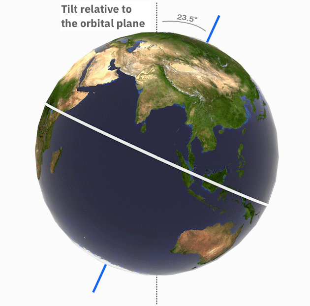 NASA, JPL
The cycle of the seasons arises because of the tilt of Earth’s axis. As the Earth goes around the Sun, the Northern Hemisphere, for example, experiences summer when it points most toward the Sun and it experiences winter when it points most away from the Sun. If Earth were not tilted at all but spun along an axis that was straight up and down, the amount of sunlight would be the same in a given place all year round and therefore there would be no seasons.
NASA, JPL
The cycle of the seasons arises because of the tilt of Earth’s axis. As the Earth goes around the Sun, the Northern Hemisphere, for example, experiences summer when it points most toward the Sun and it experiences winter when it points most away from the Sun. If Earth were not tilted at all but spun along an axis that was straight up and down, the amount of sunlight would be the same in a given place all year round and therefore there would be no seasons.
If we think of a season as lasting roughly three months, are there any climate phenomena that have timescales between the weather timescale and the seasonal timescale? The answer is, to a degree yes, there is at least one such phenomenon, known as the North Atlantic Oscillation (NAO). The NAO is a phenomenon at the interface between weather and climate that dictates variability on a monthly timescale over the North Atlantic and surrounding regions, thus from the eastern seaboard of the United States, over Greenland, to Europe, and from the Arctic region to the Canaries. Indeed, to some extent the NAO affects the weather and climate over the entire Northern Hemisphere. There is an analogue of the NAO in the Southern Hemisphere (called the Southern Annular Mode), although it has a more hemispheric extent.
So what is the NAO? It may be thought of as a north–south oscillation of the main patterns of weather variability over the Atlantic region, especially in the winter, as illustrated below:
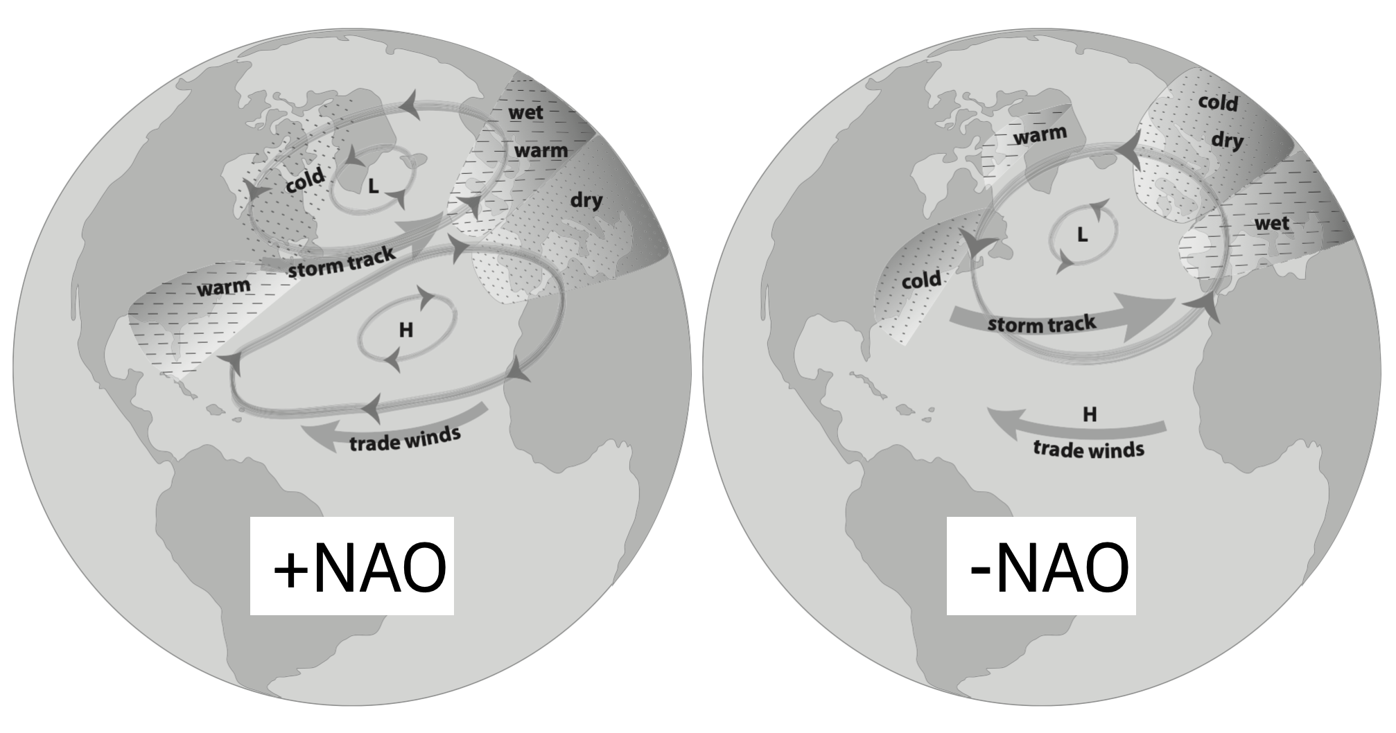
During the ‘positive phase’ of the NAO, the main path of weather systems tracks a little further north than usual. Because the air is coming straight over the ocean, it tends to be relatively warm and so brings warm, wet weather to the United Kingdom and other parts of northern Europe, with precipitation often falling as rain rather than snow in the United Kingdom, with similar effects downstream into eastern Europe and even Asia. Southern Europe and North Africa tend to have somewhat cooler weather than usual during these periods. Meanwhile, stronger northerly and northeasterly winds over Greenland and northeastern Canada bring cold, dry air to these parts, decreasing the temperature, with the eastern parts of the United States getting higher temperatures and more precipitation than normal, rather like northern Europe.
During the ‘negative phase’ of the NAO, the storm track swings southward, bringing mild, wet weather to southern Europe. During these periods, northern Europe tends to receive air that has come from the east, which, since it has come from a continental land mass in winter, tends to be very cold, with precipitation often in the form of snow. Greenland, on the other hand, is now somewhat warmer than usual. The signal of the NAO is evidently quite large and coherent and in fact accounts for about one-third of the northern Hemisphere’s interannual surface variance during winter.
The distinctive pattern of the NAO, whether positive or negative, tends to last for several days to a few weeks, perhaps a little longer than regular weather patterns, but undoubtedly the main mechanism for the NAO lies in the atmosphere itself. However, there may be a longer timescale to the NAO, as we can see below:
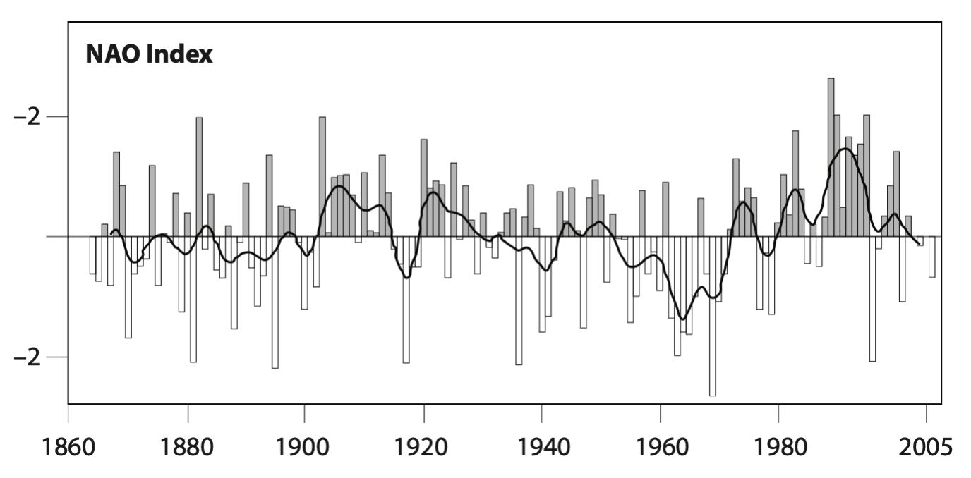
Large changes in the NAO index occur from year to year, and on the whole atmospheric behavior in one winter is largely independent of its behavior the previous winter. (The correlation in the NAO index from one year to another is only about 0.1.) nevertheless, there is some indication that there are certain periods of time when the NAO persists from year to year. For example, from about 1905 to 1915 the NAO index was largely positive. It was negative from about 1950 to 1970, and then unusually positive in the 1980s and 1990s. Among other things, the positive index in the 1980s and 1990s brought higher than usual precipitation to Scandinavia and may have mitigated the effects of global warming in the retreat of the glaciers. In contrast, over the Alps, a positive NAO index and less than normal precipitation may have worked in conjunction with global warming to cause a significant retreat of the Alpine glaciers. The Iberian peninsula and other areas around the Mediterranean also experienced drought in the late twentieth century.
It is an open question whether such long periods of persistent behavior are much more than the random variations of a chaotic system (rather like throwing six sixes in a row with a die) or whether they have a specific cause, most likely in the ocean. Why is the cause most likely in the ocean? It is because the timescales of the interannual variability correspond most closely to the timescales occurring in large-scale ocean dynamics. The dominant internal dynamics of the atmosphere are most likely too short to produce coherent dynamics that last over decadal timescales, whereas the dynamics of land ice sheets, or of changes in insolation at the top of the atmosphere because of orbital variations, are too long. One possibility is that volcanoes can have a climatic effect on the decadal timescale, but the correlation of the NAO with volcanoes is small. So let us look at the role of the ocean.
Oceanic Influence on Midlatitude Climate Variability
The ocean has one unambiguous influence on midlatitude (‘middle’ latitudes that are neither tropical nor polar) climate variability and a number of more ambiguous influences. The unambiguous influence comes from the fact that the heat capacity of the ocean is much greater than that of land. It takes a much longer time to heat up or cool down the ocean than it takes for the weather and seasons to change. So when the land surface is hot, the ocean cools it down by absorbing heat; when the land surface is cold, the ocean warms it up by releasing heat. This means that the ocean moderates climate.
For an example of this, take two cities: San Francisco and New York. The two cities have similar latitudes (San Francisco is at about 38°N and New York is at about 41°N) and both are on the coast, yet we see from the figure below that the range of the annual cycle of temperatures is much larger in New York—the highs are higher and the lows are lower.
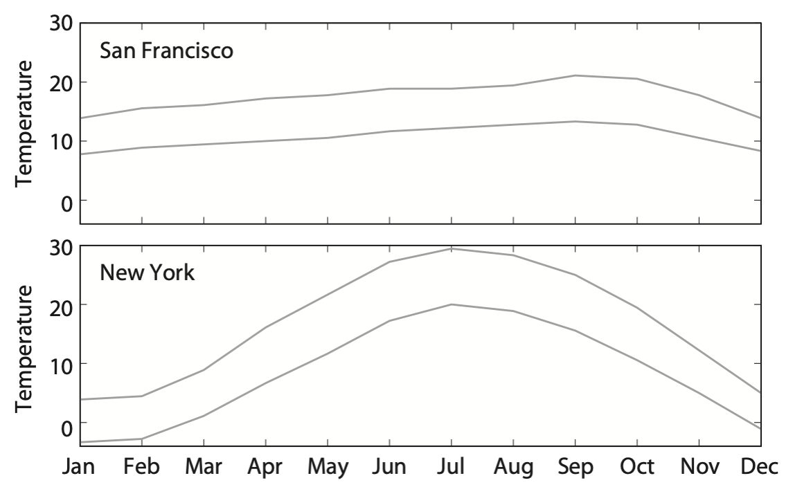
The difference is mainly caused by the fact that the climate of San Francisco is maritime, meaning that it is influenced by the ocean, whereas the climate of New York is, in spite of it being on the Atlantic coast, essentially continental. A city that is truly land-locked, such as Moscow, has a climate much more like New York than San Francisco. New York’s climate is continental because the mean winds come primarily from the west, so they blow over land and take up its temperatures before they reach the city. In contrast, the winds have blown over the Pacific ocean before arriving at San Francisco.
The more ambiguous effect of the ocean on midlatitude climate concerns the relationship between fluctuations in the sea-surface temperature (SST) and the state of the atmosphere in midlatitudes, and in particular for the Northern Hemisphere the state of the NAO. Certainly, variations in the SST and the overlying atmosphere are related. To be specific, let us focus on the North Atlantic and the NAO, but similar effects apply to other regions of the world’s ocean. It turns out that a common pattern of SST variability in the North Atlantic winter is a tripole. Rather like the NAO itself, the tripole commonly exists in one of two phases. In one phase, the pattern consists of a cold anomaly in the subpolar North Atlantic around Greenland, a warm anomaly in the middle latitudes off the Atlantic seaboard of the United States, and a cold subtropical anomaly between the equator and 30°N, concentrated most in the eastern Atlantic. Is the SST pattern created by the pattern of variability of winds and temperature in the atmosphere, or does the SST pattern determine the variability of the atmospheric winds and temperature? It may of course be a chicken-and-egg problem, with one pattern leading to the other, which then reinforces the first pattern, and so on. How are we to determine the answer? One way is to see if we can determine if variations in the atmosphere unambiguously lead those in the ocean, or vice versa. If it is the former case, then it seems likely that the atmosphere is driving the ocean, rather than vice versa.
Careful observational analysis in fact suggests that the basic pattern of SST anomalies is created by air–sea heat exchanges and the wind-induced near-surface ocean currents associated with the NAO. It seems that the correlations between atmosphere and ocean are strongest for atmospheric patterns that exist before the SST variability by a few weeks. This means that large-scale SST patterns are responding to atmospheric forcing, rather than causing the atmospheric patterns. Put simply, the atmosphere leads the ocean.
However, rather intriguingly, that may not be the whole story, although the reader should be warned that the situation is far from settled and is an active topic of research. At still longer timescales, there is some evidence that a large-scale, pan-Atlantic SST pattern actually precedes the atmospheric NAO pattern by up to about six months.Czaja and Frankignoul, Observed impact of Atlantic SST anomalies on the North Atlantic Oscillation, 2002. It is possible that the ocean’s own internal circulating variability could influence the NAO, giving it more long-lived features or persistence than it would otherwise have.
El Niño and the Southern Oscillation
El Niño is the largest and most important phenomenon to global climate variability on interannual timescales. It’s also fundamentally both an atmosphere and ocean phenomenon. El Niño is defined by an anomalous warming of the surface waters in the eastern equatorial Pacific, most pronounced just off the coast of Peru but extending westward to the center of the Pacific Ocean.
El Niño is often called ‘the El Niño—Southern Oscillation’ or ENSO. The Southern Oscillation is the atmospheric part of the phenomenon, and El Niño is the oceanic component; ENSO is the combination.
Every few years the temperature of the surface waters in the eastern tropical Pacific rises quite significantly. The strongest warming takes place between about 5°S and 5°N, and from the west coast of Peru (a longitude of about 80° W) almost to the dateline at 180° W, as illustrated below:
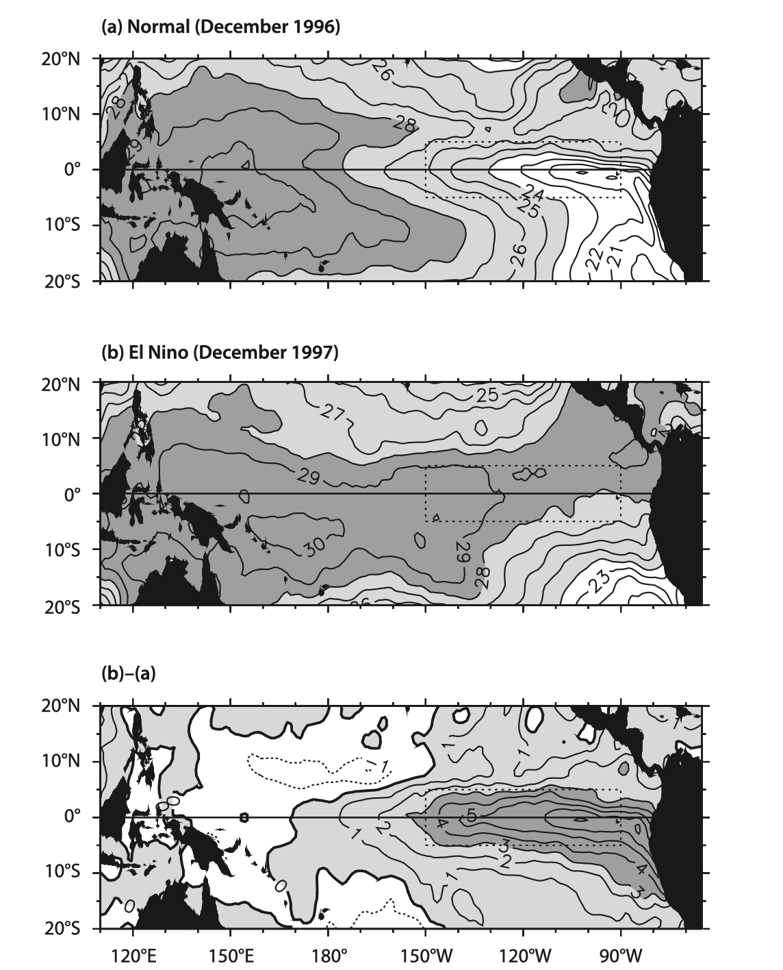
This region usually warms by 6°C during an El Niño year compared to a non–El Niño year. The warmings occur rather irregularly, but typically the interval between warmings ranges from three to seven years:
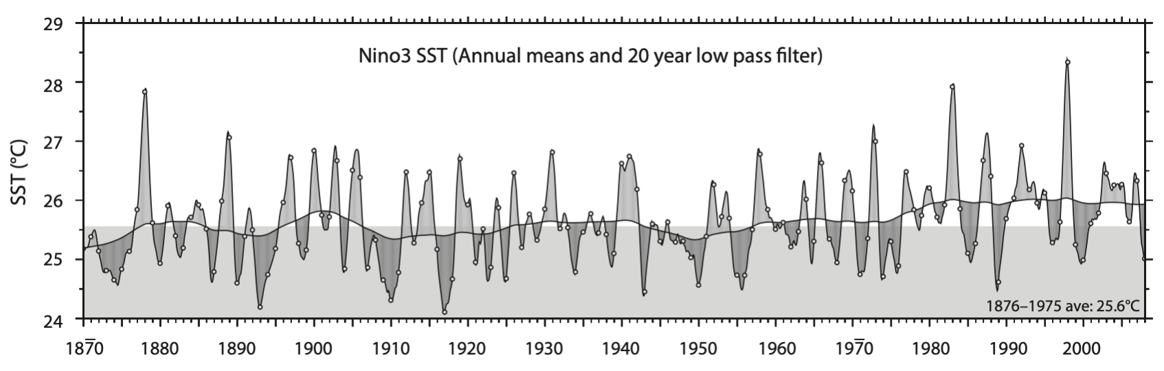
The warmings have become known as El Niño events, or even (with a little violence to the Spanish language) El Niños. The name derives from the fact that the warm waters off Peru appear at about Christmas time, and the name El Niño is Spanish for the Christ Child. The warmings typically last for up to a year, sometimes two, and appear as an enhancement to the seasonal cycle, with high temperatures appearing at a time when the waters are already warming. Although there is no universally agreed-upon definition of an El Niño, an event is often regarded as having occurred when there is a warming of at least 0.5°C averaged over the eastern tropical Pacific lasting for six months or more.Trenberth, The definition of El Niño, 1997. Rarely can a year be described as truly normal; rather, the ocean temperatures tend to fluctuate between warm El Niño years and years in which the equatorial ocean temperatures are colder in the east and warmer in the west, with those years that are particularly anomalous this way having become known as La Niña events (Spanish for ‘the young girl’). El Niño and La Niña events are thus opposites of each other: El Niños are warm, La Niñas are cold. We have direct observational evidence of El Niño and La Niña events for more than a century, but the events have almost certainly gone on for a much longer time, perhaps millennia or longer. We know this through a variety of proxy records including tree rings and corals.
The atmospheric part of ENSO, the Southern Oscillation, is fundamentally about a change of winds and pressure across the whole Pacific. During an El Niño the easterly (blowing from the east) trade winds weaken and during a La Niña the trade winds strengthen. Winds and pressure are usually very closely related and historically the Southern Oscillation was quantified as the pressure difference between Darwin, Australia (12°S, 130°E), and Tahiti (17°S, 150°W), an island in the Pacific. (There is nothing truly special about these locations vis-à-vis ENSO, but pressure measurements have been made there for a long time.) We'll explore this combined atmosphere-ocean phenomena further below.
How ENSO Works
Before we go further into learning how ENSO works, it’s helpful to see what an El Niño—La Niña cycle looks like. Watch this high-resolution ocean computer simulation below:
If we sketch out the normal conditions in the tropical Pacific, they would look like this:
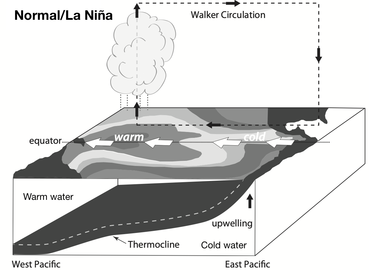
Starting at the ocean surface there is a warm pool of water north and east of Australia and centered over the equator. There are easterly winds blowing along the surface of the ocean (white arrows). If we look below the surface we see relatively warm water in the West Pacific and cold water in the East Pacific, with the layer of water called the ‘thermocline’. There is ‘upwelling’ of cold water in the east up to the surface. If we look in the atmosphere, we see convection and clouds in the west. We also see winds that circulate in an approximately closed loop: easterly along the surface of the ocean, upwards in the West Pacific, westerly high up in the atmosphere back across the Pacific, and back down again in the East Pacific. This wind pattern is called the ‘Walker Circulation’ after the British meteorologist Gilbert Walker, who described it in the 1920s.
La Niña is actually just a strengthening of these normal conditions sketched out above. Stronger winds bring up colder waters in the East Pacific and keep the convection and rain in the West Pacific.
El Niño conditions can be sketched out as:
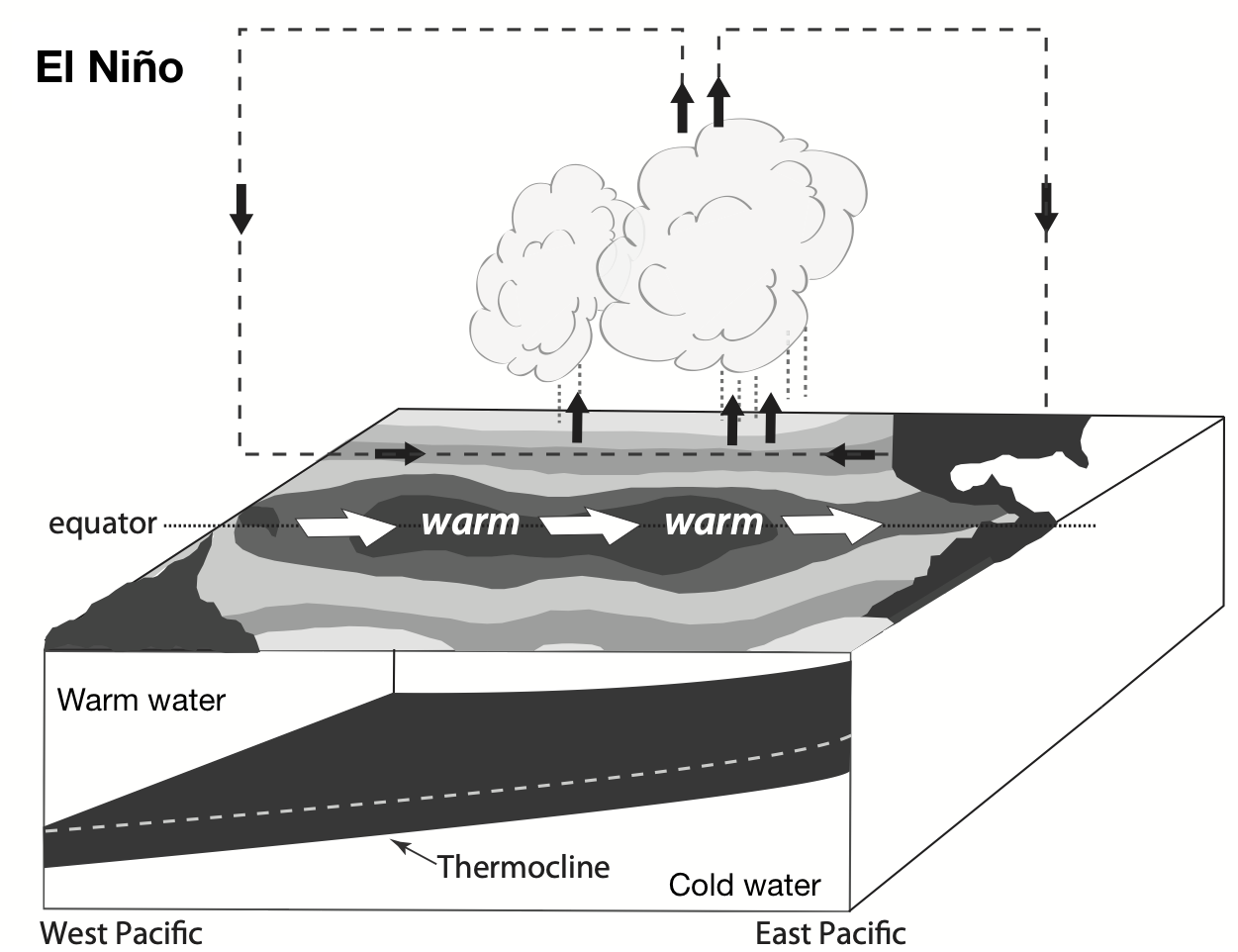
In El Niño the trade winds along the surface weaken and reverse (white arrows). This leads to warm water moving out over the center of the Pacific and an expansion of the warm water below the surface into the East Pacific. The tropical convection shifts towards the center of the Pacific, following the warm surface waters.
Local Effects of ENSO
El Niño brings significantly warmer water to the eastern tropical Pacific, and this water spreads both north and south along the coast, giving a detectable signal in the SST as far north as California and Oregon. By changing the temperature of ocean water, ENSO changes Pacific marine life: warm-water species have an extended range of habitat, whereas cold-water species try to move poleward or into deeper water, and the reduced upwelling off the South American coast produces fewer nutrients, fewer fish, and fewer sea-birds that feed off the fish. The shift of fish populations is a problem for the fishing industry, if only because the species tend to move away from established fisheries, and overall there is a loss of commercially important species. Pinnipeds (e.g., fur seals and sea lions) are also affected as far north as California because they may have difficulty finding adequate food supplies. Coral bleaching (the whitening of corals because of the loss of or changes in the protozoa living within them) in the Galapagos also occurs in El Niño years.
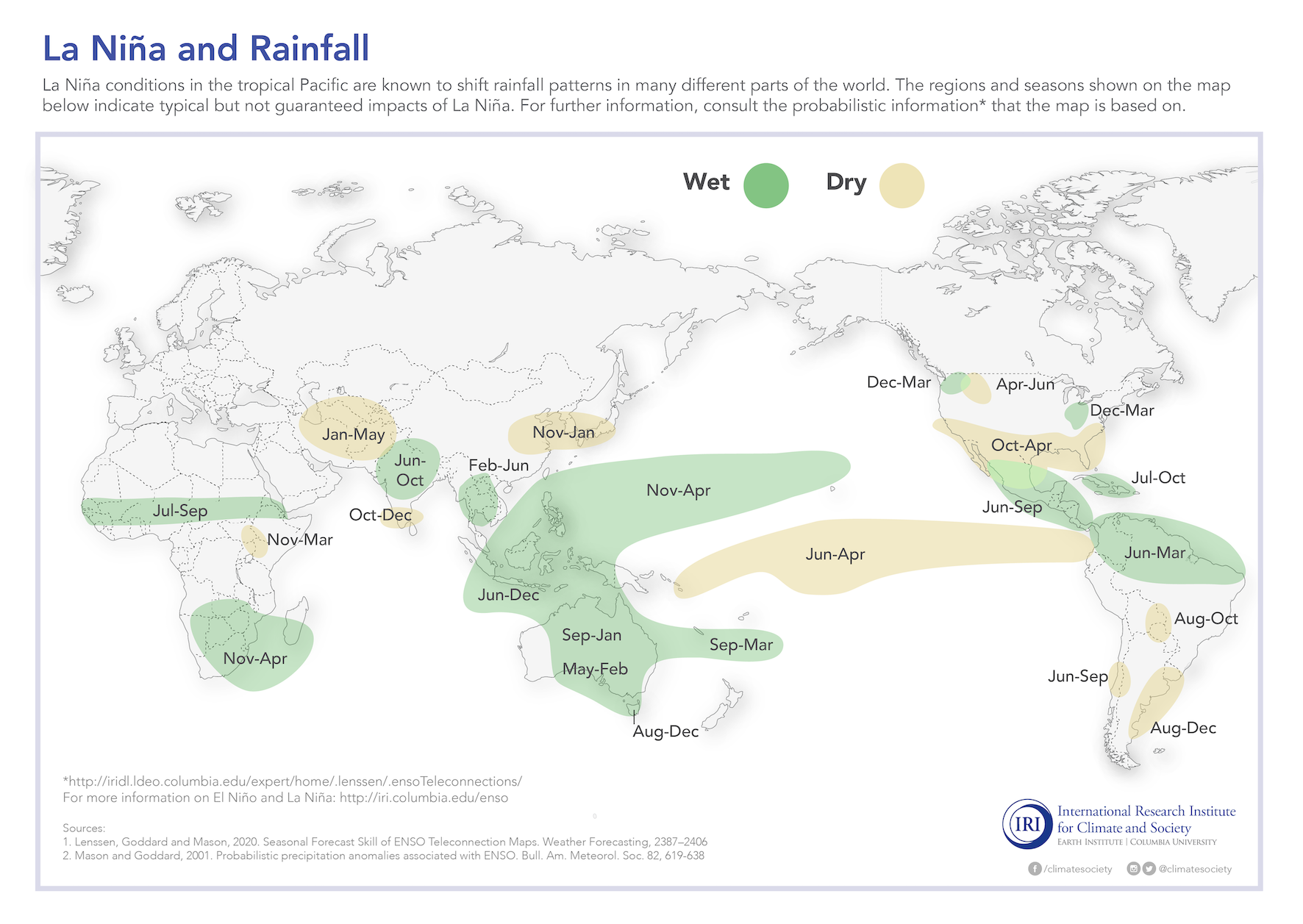
The warm ocean also affects the atmosphere above it. During a warm event, the main convective areas move eastward, and the western parts of South America, especially close to the equator in northern Peru and Ecuador, experience significantly more rainfall, especially from December to February, when ENSO events typically reach their peak. Significant flooding may occur when the event is a strong one. In contrast, northern Australia and the Indonesian archipelago experience significantly less rainfall than normal throughout the entire region and for an extended period of time. During a La Niña, the situation is almost reversed, with warmer and wetter weather in the Indonesian archipelago and northern Australia and generally cooler and dryer weather in coastal Peru and Ecuador.
Distant Effects of ENSO
Just looking at the figures above it can be hard to see how ENSO could have many non-local consequences, but it does. One overall effect is that in an El Niño year, the globally averaged surface temperature can be as much as 0.5°C higher than the years before and after, and this increase is accounted for by the fact that the surface temperatures in the eastern tropical Pacific can be several degrees higher than normal.
ENSO can have a powerful impact on where storms go outside the tropics. All the rising air in the convection depicted in the sketches above generates enormous waves in the atmosphere. A conceptual drawing of such ‘Rossby’ waves is shown below; in reality they are circular instead of ocean-wave-like, but their size is accurately drawn below.
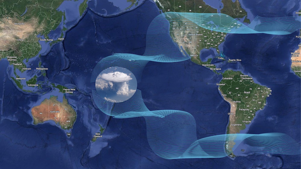
These huge waves interact with the storm track, pushing it around and changing its strength. Because ENSO changes the location where convection happens and thus where waves are generated, this results in shifts in the location and strength of the storm track.You can see videos of more accurate Rossby waves and learn more about how they impact the storm track here. And if the storm track is changed, that means that precipitation changes as well. For example, during a La Niña the winds shift most of the tropical convection westward, which changes the location of the Rossby waves, which pushes the storm track on average towards the poles, which can lead to drought in parts of North and South America.
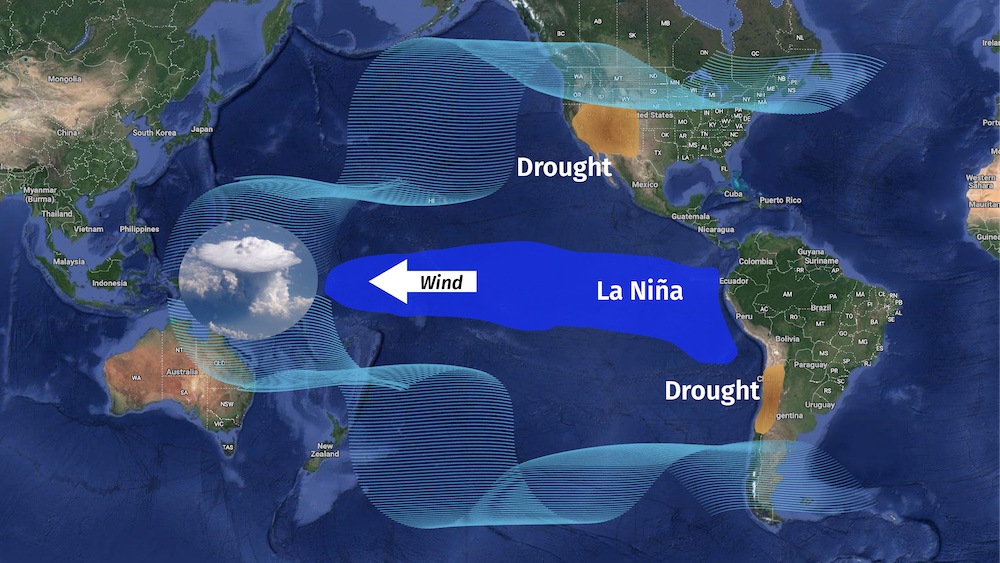
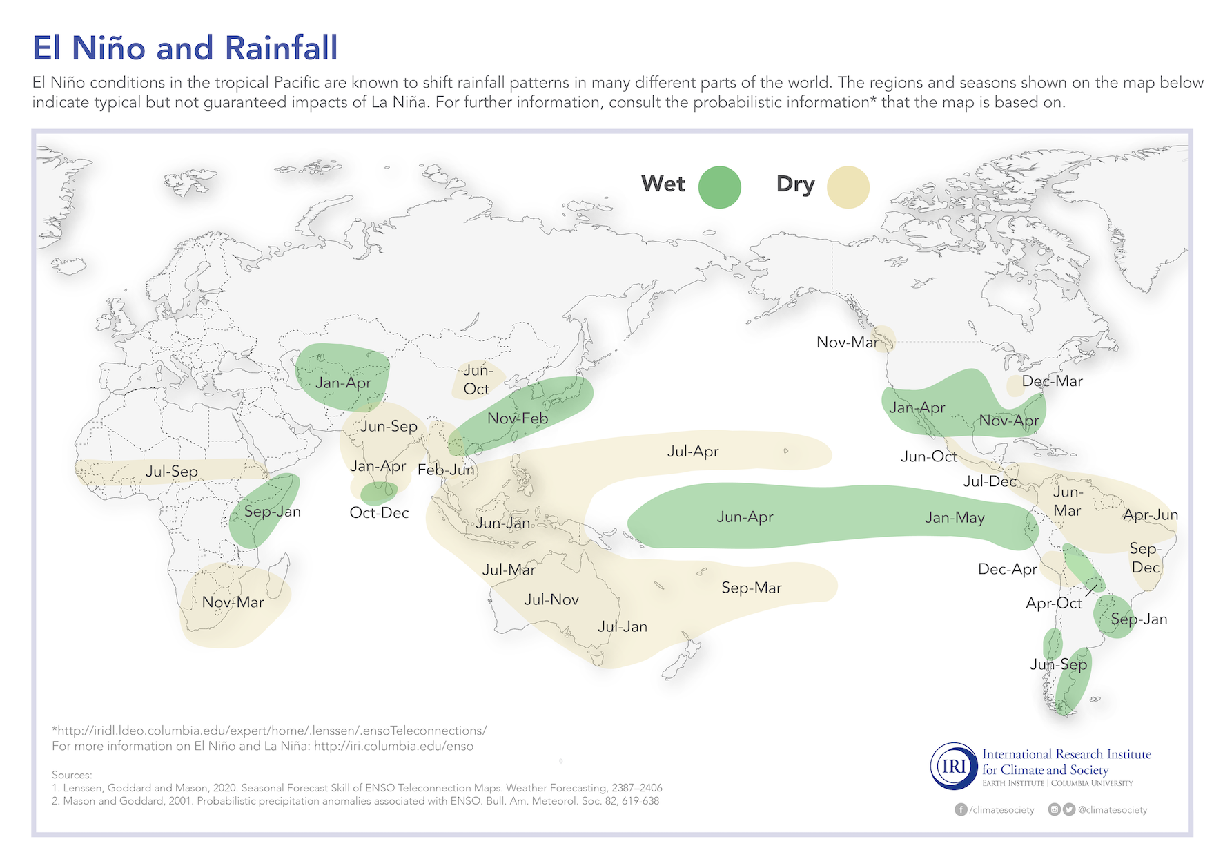
The two figures below summarize, on average, how rainfall changes during El Niños and La Niñas. ENSO is a tropical Pacific phenomenon, yet it changes precipitation well outside that region.
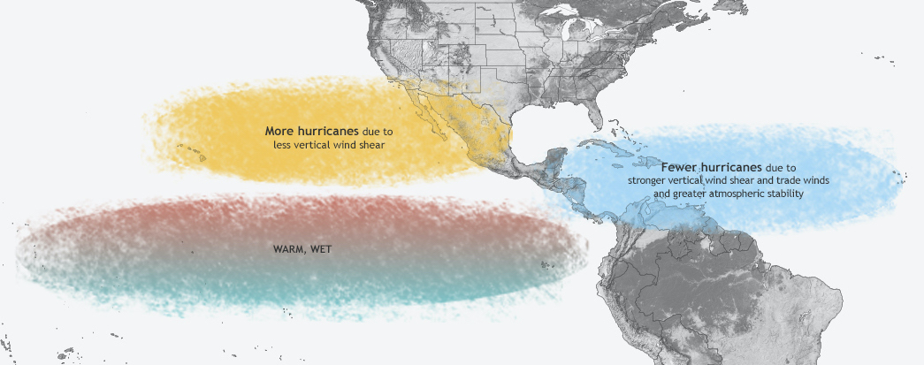
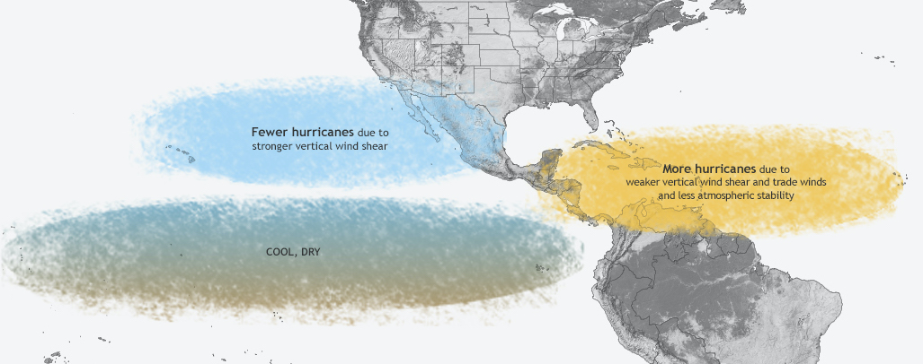
Another robust nonlocal effect is that ENSO affects hurricanes across the Pacific and Atlantic. El Niño favors stronger hurricane activity in the Pacific, and suppresses it in the Atlantic. Conversely, La Niña suppresses hurricane activity in the Pacific, and enhances it in the Atlantic. ENSO does this by changing the conditions that support hurricanes. El Niño creates air circulations that limit convection in the Atlantic while La Niña creates air circulations that encourage convection in the Atlantic. Hurricanes can also be torn apart by winds at the surface and upper atmosphere that go in opposite directions, called ‘wind shear’. ENSO also affects wind shear in the Atlantic and therefore hurricanes in the Atlantic. The figures below summarize the typical specific influences for El Niño and La Niña.
Global Climate Variability
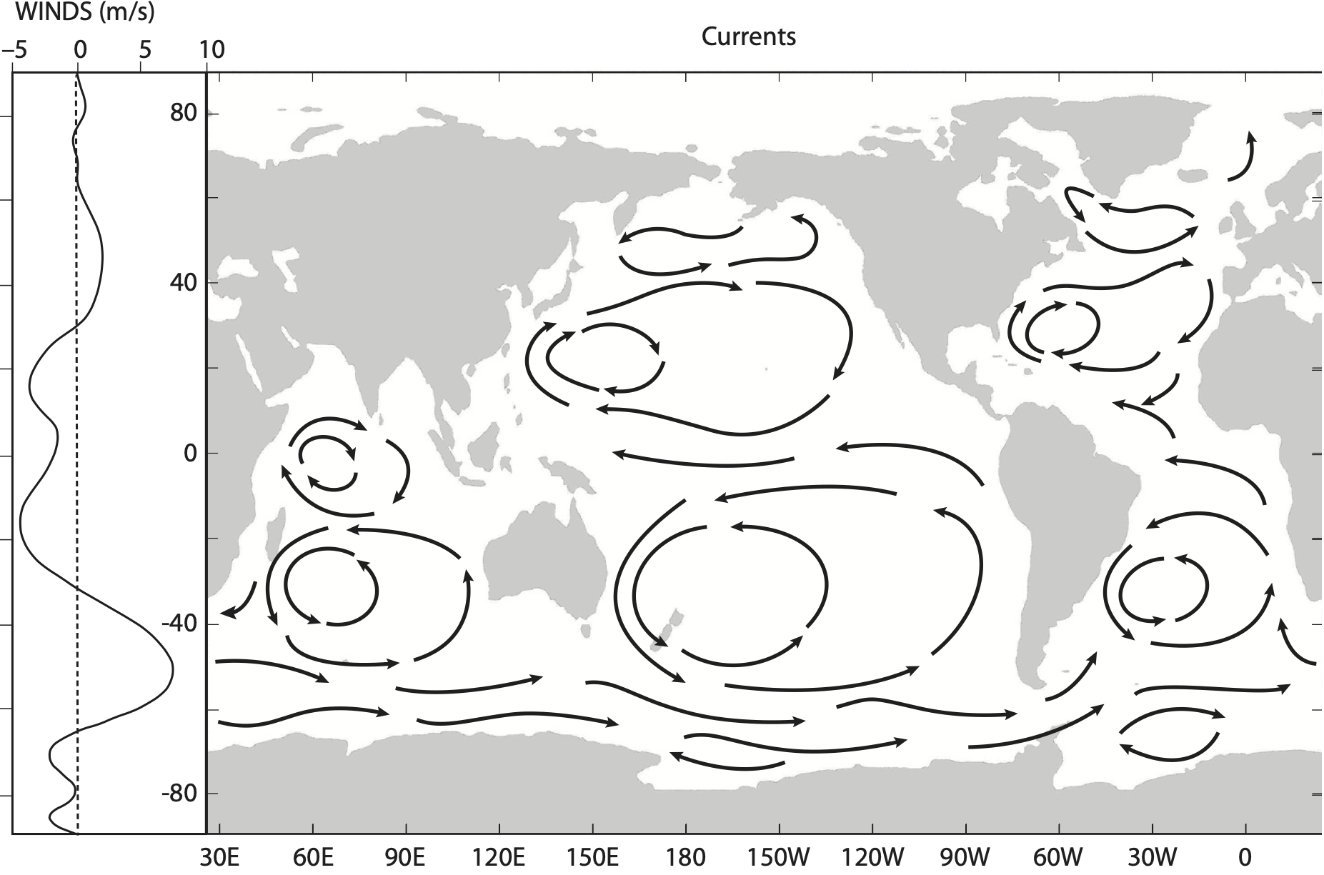
Besides the ocean’s role in moderating climate, it also redistributes heat in a global large-scale circulation. This circulation has two components: a mostly near-surface ‘gyre’ circulation and a deep ‘overturning’ circulation. The gyre circulation is driven by differences in the average direction of atmospheric winds and it creates circular gyres in ocean basins:
In contrast, the deep overturning circulation is driven by differences in the density of water in different parts of the ocean. A simplified schematic of this circulation is given below, with important areas of water sinking indicated by gray circles.
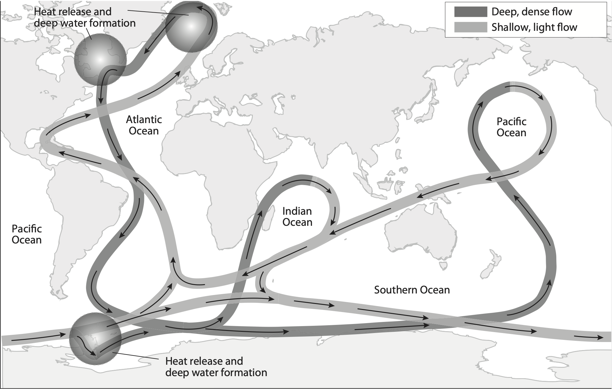
The details of the ocean circulation are fairly complex and for our purposes it’s most important to know that as the ocean circulates and redistributes heat, it creates climate variability on timescales that are much longer than atmospheric timescales. This is due to the simple fact that water is denser and slower moving than atmospheric gases. Some surface parts of the ocean exhibit multiyear and decadal variability while the deep overturning circulation takes hundreds of years to fully adjust to a big change. This means that we can expect there to be long timescale fluctuations in climate that are part of the natural variability of the ocean as it circulates heat around the planet.
Variability in climate comes from two kinds of sources, those that are ‘external’ to the climate system and those that are ‘internal’ to it. ‘External forcings’ are things that affect climate, usually the radiative energy balance of the planet, and come from ‘outside’ it. Over the past several thousand years the two most important external forcings are greenhouse gases that warm Earth and very large volcanic eruptions that spew out ash into the stratosphere, which blocks sunlight and cools Earth. ‘Internal climate variability’ consists of the climate fluctuations that come from the natural variability of the atmosphere and ocean; this includes all the atmosphere and ocean phenomena that we have discussed in this chapter along with a few other phenomena that we didn’t have space to discuss.
If we want to completely explain all the climate variability Earth has experienced, we have to consider both external forcings and internal variability. Let’s look at an observations-based estimate of global mean land temperature from about 1830 to approximately the present, compared against an estimate of external forcings:
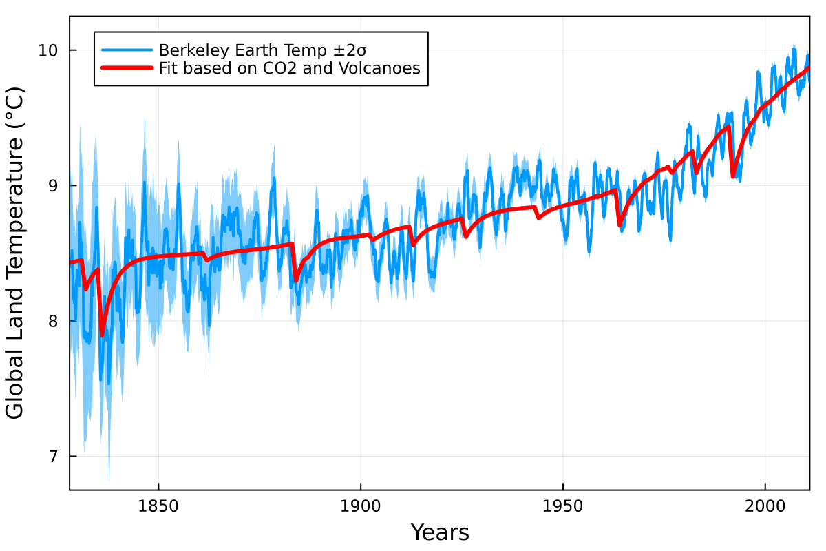
We can see that the trend and large drops match the primary external forcings of CO2 and major volcanic eruptions, yet there is variability that cannot be explained by these forcings. There is annual variability that can be explained by ENSO or atmospheric phenomena like the NAO. And there is decadal variability that can be explained by changes in ocean circulation. One of the primary tasks of climate science is to piece together the causes of all the variability and thereby better understand how the climate system works.
\(\Uparrow\) To the top
\(\Rightarrow\) Next chapter
\(\Leftarrow\) Table of contents