Predictability of Weather and Climate
Revised and adapted from ‘Atmosphere, Clouds, and Climate’, David Randall (2012)
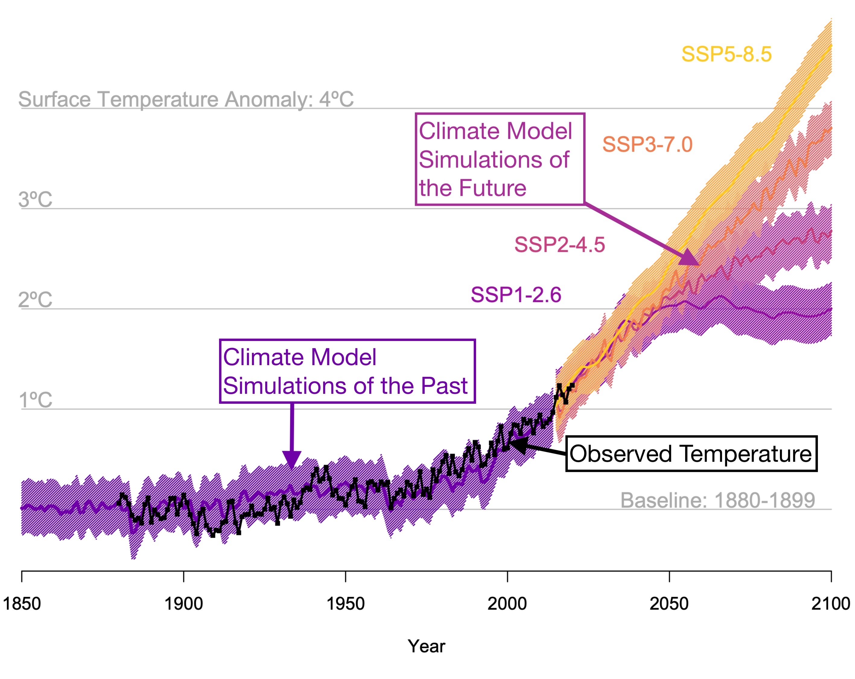
How can we predict future climate? Our textbook’s motivating figure, below, shows predictions decades out into the future. How is this even possible? To answer this question, let’s actually first discuss how weather forecasts are made.
How Weather Forecasts are Made
Weather forecasts are all around us, on television, the radio, and the web. Where do they come from? Forecasts are made by solving equations that predict how the weather will change, starting from its observed current state. The equations comprise ‘mathematical models’ that can be solved only by using very powerful computers. The models predict the winds, temperature, humidity, and many other quantities. The first such models were created in the 1950s. Through intensive worldwide efforts, driven partly by friendly competition among forecast centers, the forecast models have been refined, year by year, and have now reached an advanced state of development.
In practical terms, a forecast model is a large computer program, containing a few million lines of code. The formulation of a forecast model is based on physical principles, such as conservation of mass, momentum, and energy. The spatial structure of the atmosphere is represented in a model by using grid points that, in the most advanced models, are now (in 2022) about 10 km apart in the horizontal and variably spaced vertically, from a few meters near the surface to several hundred meters in the upper troposphere and stratosphere. The grid spacing of the model is often referred to as its ‘resolution’. A high-resolution model is one with many closely spaced grid points. Higher resolution requires a more powerful supercomputer but it is usually (though not always) more accurate.
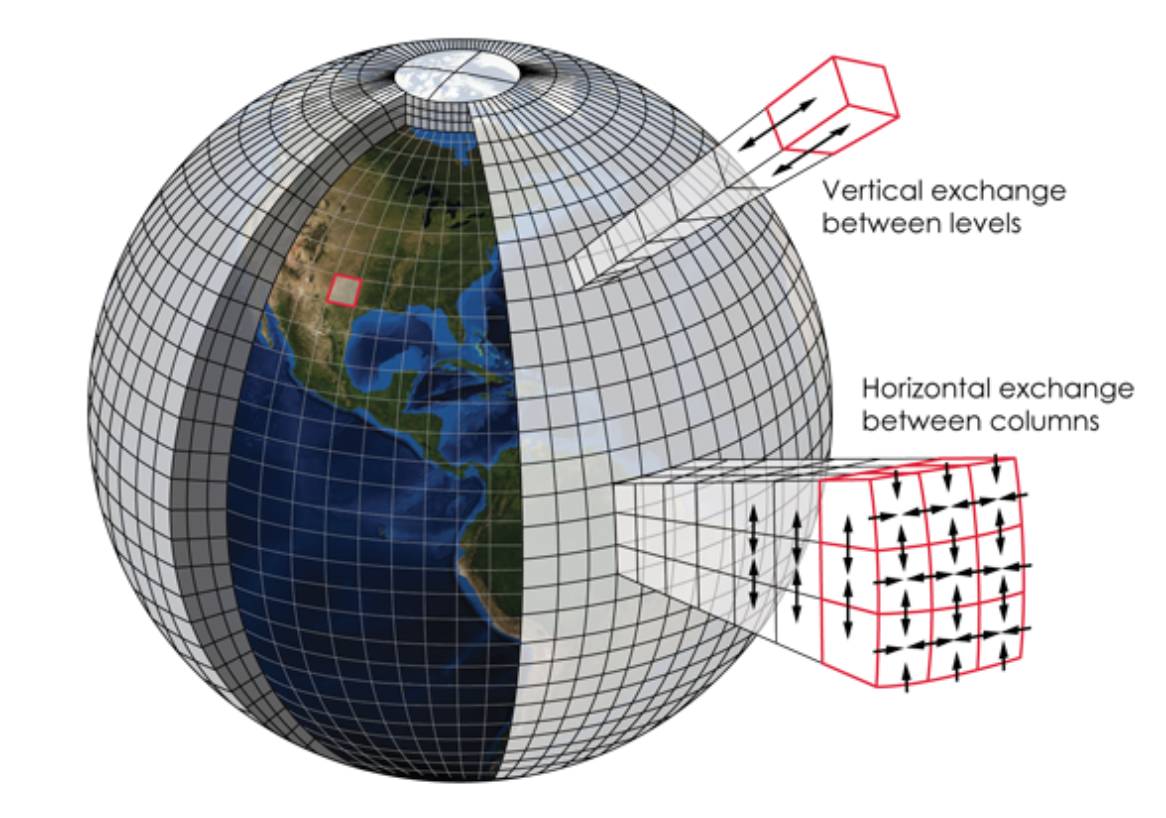
The global atmospheric models used to simulate climate change are essentially the same as the global weather forecast models, except that the climate models use lower resolution so that they can run faster and over longer time periods. Today, a typical global atmospheric model used for climate simulation has grid points that are horizontally spaced by 50-100 km.
A forecast starts from the observed weather situation at a given moment in time. The gridded data used for this are called the ‘initial conditions’. The data needed to create the initial conditions are obtained from a huge international observing network that includes surface stations, weather balloons, aircraft, and satellites, all of which are developed and operated under government funding. The data cannot be directly acquired on the regular grid used by a model, because weather stations, weather balloons, and satellite overpasses are irregularly situated in both space and time. The data are electronically gathered and gridded at the operational forecast centers, which also develop and run the forecast models. The models themselves are used to combine the many different types of data, collected at inconvenient places and times, into a coherent, self-consistent, quality-controlled, and gridded snapshot of the atmosphere that can be used as the initial conditions for a forecast. This very complex process is called ‘data assimilation’.
The observing systems and forecast centers are operated by wealthy, technologically advanced nations and consortiums of nations. They are highly organized, quasi-industrial enterprises and adhere to strict and challenging schedules, so that the models can be run and forecasts can be delivered to the public every few hours.
When a forecast model starts up, it reads in the initial conditions and then predicts how the atmosphere will change over a short ‘time step’ of a few minutes. Then it takes another time step, and another, until the forecast has advanced over as much simulated time as required by the human forecasters—usually a few days to two weeks. The results are saved frequently as the model steps forward to create a record of the evolving state of the atmosphere over the period of the forecast. For reasons discussed later, it is now standard practice to run each forecast dozens of times. The simulations have to finish quickly enough to fit the schedule for releasing new forecasts.
When the computer-generated forecast is ready, it is analyzed by human forecasters at the national forecast centers, at local weather service offices, and sometimes also at media outlets. The humans use their judgment and experience to add value. Although human forecasters sometimes condescendingly refer to the model-generated forecast as the ‘numerical guidance’, it is fair to say that, with rare exceptions, the forecast information that is provided to the public comes primarily from the forecast models.
Weather forecasting is a tough business. Forecasts are methodically compared with what really happens, and errors are quantified through detailed analyses. This is especially true for the attention-getting forecasts that are badly wrong. Over the months and years, statistics are compiled to evaluate a model’s forecast skill. Forecast centers from around the world compete with each other, and over the past few decades the performance of the models has improved gradually but impressively. For example, 5 day forecasts are currently as good as 3 day forecasts were in the 1990s, and 7 day forecasts are currently as good as 5 day forecasts were in the 1990s. The improvements come from better data that can be used to make better initial conditions, and also from major improvements to the models themselves. Model improvements are achieved partly by adding more grid points and also, importantly, by improving the equations that are used to represent the physics of the atmosphere.
How Predictable is the Weather?
Are there limits to how good the forecasts can become? It turns out that, for fundamental physical reasons that are unrelated to any specific forecast method, it is impossible to make a skillful weather forecast more than about two weeks ahead.
As a first step toward understanding why, it is useful to consider three broadly defined sources of forecast error. First of all, there are errors in the initial conditions. The instruments (e.g., thermometers) used to make the various measurements are not perfect. There are spatial and temporal gaps in the data, even in this era of weather satellites. The larger spatial scales tend to be relatively well observed because they cover a larger area and so are sampled by more instruments. Smaller scales are less well sampled, and many small-scale weather systems are not observed at all. As a result, the most serious errors in the initial conditions tend to be on the smallest spatial scales that can be represented on a model’s grid. We will come back to this point later. As the years go by, the observing system improves, and so the quality and quantity of the data that go into the initial conditions get better and better. Over the past 50 years or so, the gradual introduction of satellite data has enabled dramatic improvements in the accuracy of weather forecasts, especially for the Southern Hemisphere.
The second source of forecast errors is imperfections of the forecast models themselves. The resolution of a model is limited by the available computer power. In addition, the equations of the model are not exact, especially for the parameterized processes like turbulence and cloud formation. The models are improving, year by year, but they will never be perfect.
Finally, and most importantly, our ability to predict the weather is limited by properties of the atmosphere itself. These are the most fundamental limitations because they are not related to any particular forecast model or observing system. At this point, you may be thinking of the Uncertainty Principle of quantum mechanics, which forbids exact measurements of the state of a system. The Uncertainty Principle is not important for weather prediction because there is a much larger source of uncertainty in classical physics, also intrinsic to the physical nature of the atmosphere: it is sometimes called sensitive dependence on initial conditions.
Before we talk about how sensitive dependence on initial conditions applies to the atmosphere, let’s look at an even simpler system: the double pendulum, which is just two pendulums connected to each other and swung back and forth. Below is a computer simulation of two double pendulums, one white and the other red, that are started in a very similar, though not exactly the same position.
At first the pendulums behave basically identically, but over time they diverge and end up having completely different movements. They key feature of this system is that a double pendulum does not have stable movements like a single pendulum would. Its movements are unpredictable and unstable. In the presence of instability, a small difference between two initial states can amplify with time. If we were to run a similar experiment but with single pendulums instead of double pendulums, the two pendulums would never drift further apart from each other than by the tiny difference in their initial conditions.
Many kinds of instability are at work in the atmosphere, acting on virtually all spatial scales. For example, shearing instabilities (called ‘Kelvin-Helmholtz Instability’) act on scales of meters and smaller. Such shearing instability occurs when you have large velocity differences within a ‘fluid’ like water or air. You can see this shearing instability causing chaotic fluid motions in the following experiment of a jet of smoke illuminated by a green laser; shearing and chaotic vorticies like this are occuring everywhere in the atmosphere and ocean:
In the atmosphere, instabilities at various scales interact with each other. Small-scale weather systems, such as cumulus clouds, can modify the larger scales, such as Rossby waves, and these in turn can strongly influence where and when the cumulus clouds grow. It is the combination of instability and scale interactions that leads to sensitive dependence on initial conditions.
We can see sensitive dependence on initial conditions in weather forecasts. An example is given in the form of the ‘spaghetti diagrams’ shown below:
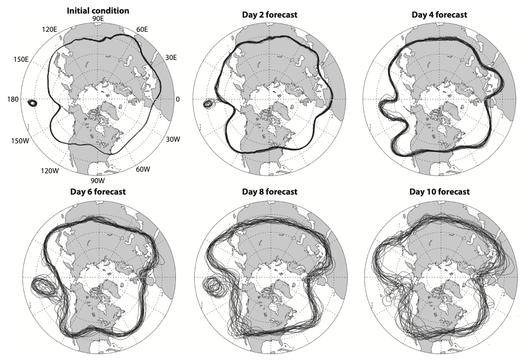
The figure shows the results of actual forecasts. For simplicity, each highly detailed forecast is represented by a single curve that shows where the height of a pressure surface in the middle troposphere takes a certain value. This is called a height contour. For each forecast, the winds would blow approximately parallel to the height contour shown, and primarily from west to east, weaving back and forth between higher and lower latitudes.
In the different panels of the figure, the forecast times shown are the initial conditions, and then every two days after that, out to ten days. For each forecast time, the plots show the results from an ensemble of 20 forecasts that are started from initial conditions that differ very slightly from those of the control run. There are 20 curves in each panel, one for each forecast. The 20 forecasts all start from almost but not quite the same initial conditions. You can tell that the initial conditions are very similar for all 20 forecasts because the contours essentially fall on top of each other in the initial condition plot shown in the top-left corner of the figure. By design, the differences in the initial conditions are so small that the accuracy of the observations is not sufficient to enable us to determine which one is closest to the true state of the atmosphere.
Two days into the forecast, the 20 predicted configurations of the weather are in pretty good agreement, except for a small region in the central Pacific, where the ensemble members differ considerably. The generally good agreement among the ensemble members gives confidence that the forecasts are reliable, and in fact the statistics show (and we know from common experience) that two-day forecasts are usually pretty good. After four days, the disagreements in the central Pacific have actually diminished, but the plots have become ‘fuzzy’ virtually everywhere, because the different forecasts are beginning to disagree noticeably everywhere. By day 6, large disagreements have reappeared in the central Pacific, and the forecasts are also disagreeing quite a bit over northern Europe and eastern Asia. By day 10, the ensemble members have diverged so much that they provide little guidance on what the real atmosphere will do; they have become fairly useless.
This example shows that after about a week, very small differences in the initial conditions can lead to large changes in forecasts performed with the same model. The details vary from case to case, and to some extent with season, but the basic pattern of gradually increasing forecast error is seen every time a forecast ensemble is run.
Our understanding of how very small differences in the initial conditions can lead to large changes in forecasts comes largely from the work of Edward Lorenz, as first reported in an article titled ‘Deterministic non-Periodic Flow’, published in 1963. The title of Lorenz’s article needs some explanation. A system is said to be deterministic if its future evolution is completely determined by a set of rules. The atmosphere obeys a set of rules that we call the laws of physics. It is, therefore, a deterministic system. A periodic system (or flow) is one whose behavior repeats exactly on some regular time interval. Despite the existence of the externally forced daily and seasonal cycles, the behavior of the atmosphere is nonperiodic; its previous history is not repeated. The predictability of periodic flows is a rather boring subject. If the behavior of the atmosphere were really periodic, the weather would certainly be predictable!
How does nonperiodic behavior arise? This is where scale interactions come in. The forcing of the atmosphere by the seasonal and daily sunlight cycles is at least approximately periodic. When scales do not interact, periodic forcing always leads to a response with the same period. When scales do interact, however, periodic forcing can lead to a nonperiodic response. Nonperiodic behavior arises from scale interactions.
Lorenz (1963) analyzed an idealized set of equations, loosely derived from a very simple atmosphere model. He found that, for some values of the parameters, all of the steady and periodic solutions are unstable. The instabilities arise on different scales, and the scales interact with each other. As a result, the model exhibits non-periodic solutions; again, a periodic solution is, by definition, predictable.
The equations of Lorenz’s model are remarkably simple: \[ \displaylines{ \frac{dX}{dt}=-\sigma X + \sigma Y\\ \frac{dY}{dt}=-XZ + rX - Y\\ \frac{dZ}{dt}=XY - bZ } \] The unknown variables are \(X\), \(Y\), and \(Z\) and the parameters \(\sigma\), \(b\), and \(r\) are single values that are specified before the model is run. The system consists of three coupled first-order ordinary differential equations.
The terms of these equations that involve products of the unknowns lead to interactions among timescales (\(XZ\) and \(XY\)). Mathematically speaking, those terms are said to be ‘nonlinear’ because the product of two unknowns is a nonlinear expression. The model itself, as represented by the three equations, is also said to be nonlinear. A nonlinear model permits scale interactions. Realistic models of the atmosphere, such as weather forecast models, are highly nonlinear.
Let’s see what this model looks like when it is solved numerically on a computer. The video below shows two different computer simulations of the Lorenz model, each starting from a different initial location. The computer solves the Lorenz equations as a function of time given the initial conditions.
Note that this video only shows a projection of the Lorenz model into two dimensions (\(X\) and \(Z\)), thus making it easier to see how the simulation evolves in time. Here’s a three-dimensional plot of the ‘Lorenz attractor’ that you can see being traced out in the two-dimensional simulations above:
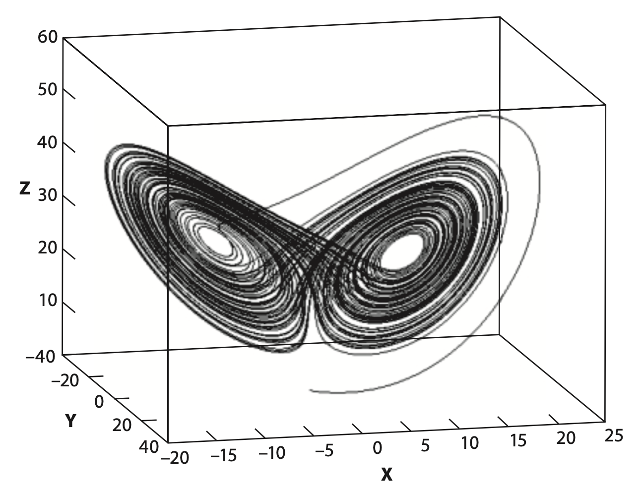
The solution of the Lorenz equations traces out a path that looks like two butterfly wings. The wings are called ‘attractors’ because the solution tends to ‘attract’ or stay close to them, while the rest of the domain is avoided. At a randomly chosen time, the probability of finding the solution near one of the attractors is high. Occasionally the solution jumps from one attractor to the other. These transitions between attractors occur somewhat randomly. Lorenz demonstrated that this simple system exhibits sensitive dependence on initial conditions, analogous to the behavior of the forecasts we saw previously.
Lorenz’s model illustrates that even a simple system that includes scale interactions can be unpredictable and chaotic. In other words, unpredictable, complex behavior is not necessarily due to complexity in the definition of the system itself.
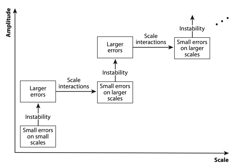
It is the combination of instability and scale interactions that limits our ability to make skillful forecasts of the largest scales of motion in the atmosphere, illustrated below. The scale interactions are essential because otherwise, for example, errors on small scales could just stay at small scales and therefore the large scales (like storm systems) would not be affected and might thus be predictable over long timescales.
We can say that sensitive dependence on past history imposes a ‘predictability time’ or ‘predictability limit’, beyond which the weather is unpredictable even in principle. This limit is a property of the atmosphere itself, and for that reason there is no way around it. No matter what method is used to make a forecast, the predictability limit comes into play. Sensitivity to initial conditions is not a limitation that is tied to numerical weather prediction or any other specific forecast method. It applies to all forecast methods because it is a property of the atmosphere.
Errors on smaller scales double (grow proportionately) faster than errors on larger scales, simply because the intrinsic timescales of smaller-scale circulations are shorter. For example, the intrinsic timescale of a buoyant thermal in the boundary layer might be on the order of 20 minutes, that of a thunderstorm circulation might be on the order of an hour, that of a winter storm might be two or three days, and that of a larger atmospheric wave that just fits on the Earth might be two weeks. Weather systems with longer intrinsic timescales are more predictable. As a result, the predictability limit is a function of scale; larger scales are generally more predictable than smaller scales.
When we reduce the errors in the initial conditions on small spatial scales by adding more observations, the range of our skillful forecasts is increased by a time increment that is approximately equal to the predictability time of the newly resolved small scales. For example, suppose that we are able to observe weather systems with intrinsic timescales of two days or longer and that we have models able to model such weather systems. By spending a lot of money, we can improve the observing system and the forecast model to permit prediction of weather systems with shorter intrinsic timescales—say, one day. This will lead to a one-day improvement in our forecast skill. Pushing the initial error down to smaller and smaller spatial scales is, therefore, a strategy for forecast improvement, but it is subject to a law of diminishing returns. Each successive refinement of the observing system and the models gives a smaller increase in the predictability time. At some point, we may choose to forego the improvement that would come from more accurate initial conditions and higher resolution models on the grounds that the benefit would be too small to justify the cost.
Quantifying the Limits of Predictability
In 1969 Lorenz outlined three distinct approaches to determine the limits of predictability.Lorenz, The predictability of a flow which possess many scales of motion, 1969. The first is based entirely on models, the second entirely on observations, and the third uses both models and observations. In the decades since Lorenz proposed these different approaches, many scientists have explored the predictability limit of the midlatitude atmosphere. For large spatial scales such as the location of large storm systems, each approach shows that the predictability limit is about two weeks.
The predictability limit exists because small errors on the smallest spatial scales can grow in both amplitude and scale until they significantly contaminate the largest scalesLorenz, The predictability of a flow which possess many scales of motion, 1969. (comparable to the radius of the Earth) in about two to three weeks. Likewise small errors on large scales can propagate down to smaller scales,Durran and Gingrich, Atmospheric predictability: Why butterflies are not of practical importance, 2014. also limiting the predictability on a similar timescale.
Some aspects of atmospheric behavior may nevertheless be predictable on longer timescales. This is particularly true if they are forced by slowly changing external influences. An obvious example is the seasonal cycle. Another example is anomalies of the average weather that are associated with long-lasting sea surface temperature fluctuations, such as those due to the El Niño–Southern Oscillation.
Climate Prediction
If weather prediction is impossible beyond about two weeks, how can climate prediction be contemplated at all? Two factors make climate change prediction possible. First, the timescales of weather and climate are very different. Forecasting multiyear average climate conditions is therefore fundamentally different than forecasting the weather. Second, the climate system responds in systematic and predictable ways to changes in the external forcing. And because the future external forcing can be reasonably predicted, this makes ‘forecasting’ the average climate under global warming possible (global warming forecasts are made for several plausible future forcing scenarios).
The predictable response to external forcing means that it is possible to make a prediction without solving an initial-value problem. A good example is the seasonal cycle. It is possible to predict systematic differences in weather between summer and winter in any given location, such as London. We have a very good understanding of why those differences occur, in terms of the movement of the Earth in its orbit around the Sun. A climate model started on January 1 from initial conditions for the atmosphere, ocean, and land surface can predict, with ease, that the average July temperatures in London will be much warmer than those of the initial conditions. In fact, it can predict that every single day in July will be warmer than January 1. That same model, started from the same real, observed January 1 initial conditions, cannot predict the weather in London on January 15.
The movement of the Earth around the Sun is very predictable. It represents a strong change in the external forcing of the climate system. The response of the climate system to that change in forcing is also predictable.
Climate prediction is possible when there is a strong, predictable change in the external forcing of the system. The ice ages are the predictable response to gradual changes in the Earth’s orbital configuration. Similarly, the ongoing warming of the climate is a predictable response to the increase of greenhouse gases in the atmosphere.
Weather prediction is very different from climate prediction because changes in the day-to-day weather are not due to changes in the external forcing, while changes in climate are. Weather prediction is limited by sensitive dependence on past history while climate prediction is not.
\(\Uparrow\) To the top
\(\Rightarrow\) Next chapter
\(\Leftarrow\) Table of contents