The Present and Future Carbon Cycle
Revised and adapted from ‘The Global Carbon Cycle’, David Archer (2010)
We’ve learned how CO2 acting through the carbon cycle has affected climate over very long geological time scales. Now let’s look at the recent past and into the future.
Historic CO2 Levels
We have two kinds of direct measurements of past CO2 levels in the atmosphere. One comes from ancient bubbles of air trapped in the ice sheets of Antarctica and Greenland; we can measure the gases in these bubbles if we extract a core of ice and take it back to a lab and melt it down inside a chamber. The other measurements we have of past atmospheric CO2 were made with special-built equipment by David Keeling starting in 1957, which we read about in Chapter 1. If we stitch these two kinds of records together, this is what we get for atmospheric CO2 over the past 800,000 years:
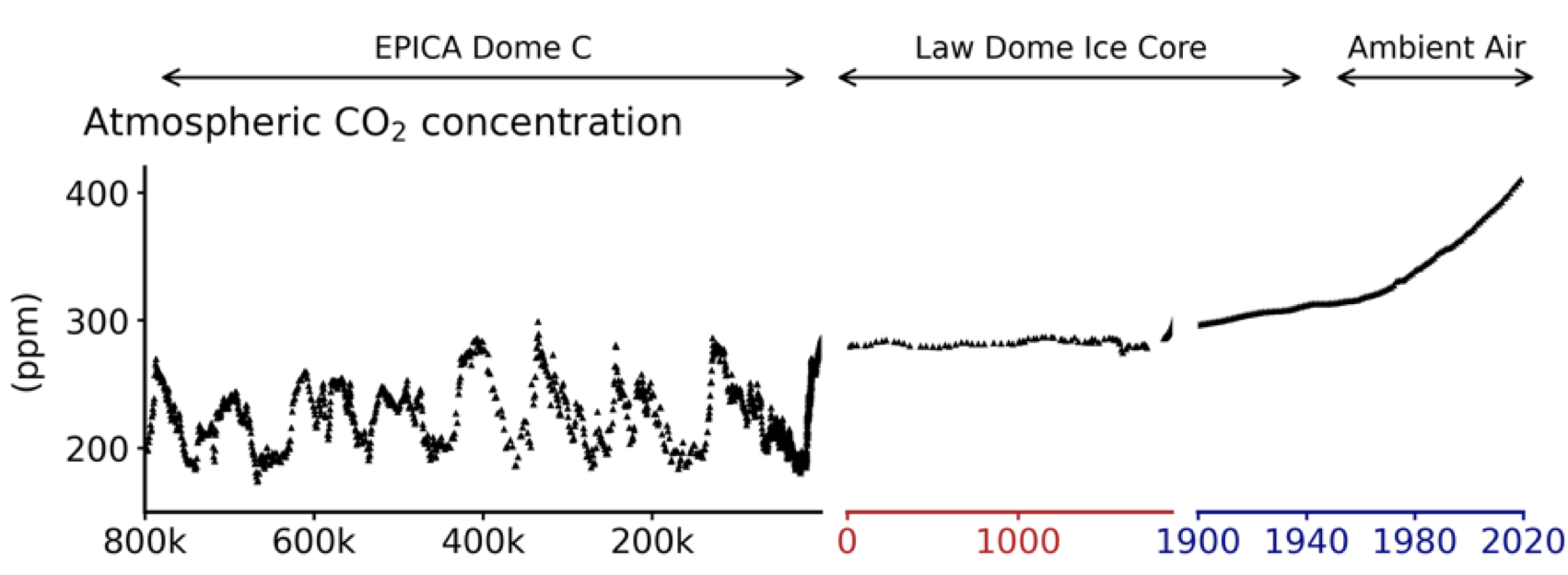
We see fluctuations between 180 ppm and 280 ppm during the ice age cycles, followed by a steady ~280 ppm through the past 1900 years, and then a strong rise up to the present ~415 ppm (the 2022 level). The story of what caused the ice age fluctuations in CO2 turns out to be fairly complicated and so we won’t cover that here. But the rise in CO2 over the past 200 years or so is far better understood because we have so much more data.
Over the past decade humans have been emitting about 38 Gton CO2 per year (or about 10 Gton C per year, counting only the carbon atoms and not the oxygen atoms). This is mostly a carbon flux from the solid Earth, from combustion of fossil fuels and cement manufacture, supplemented by the destruction of carbon biomass on land. Our carbon emissions are 100 times larger than the analogous natural carbon flux from the solid Earth to the atmosphere, the degassing of CO2 in volcanic gases and deep sea hot spring fluids (about 0.1 Gton C per year). The human-associated emission rate has been growing since the 1800s, with only minor short-term decreases for major crises like the COVID-19 pandemic:
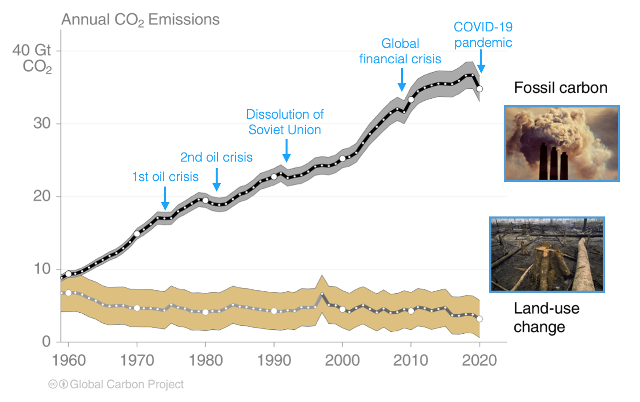
Prior to about 1950, the largest source of human-caused CO2 emissions came from ‘changes in land use’ (e.g., deforestation or replacing grasslands with cities). Natural forests or grasslands hold far more carbon than agricultural fields or human cities, so the destruction of these landscapes and burning or decomposition of the trees and plants leads to CO2 emissions that aren’t reversed. After about 1950, fossil fuel emissions have increasingly dominated the total human emissions, as we can see in the figure above.
Over the past decade (2011-2020), carbon has been increasing in the atmosphere by about 5 Gton C per year.Friedlingstein, et al., Global Carbon Budget 2021, (2022). This is half the rate of the human emission of CO2, about 10 Gton C per year. So where is the rest of the human-emitted carbon going? There are two possibilities: carbon can go into the land biosphere or it can go into the ocean.
It is much easier to measure the rate at which fossil fuel CO2 is being dissolved in the ocean than it is to measure land uptake. The chemistry of the ocean is smoother, more homogeneous, so that even a ‘transect’ of measurements from a range of depths along a ship cruise track can reveal smooth large-scale patterns in temperature, chemical concentrations, and so forth. The land surface, in contrast, is extremely heterogeneous. To measure a trend in the amount of carbon in all the soils on Earth would require an almost unimaginable number of soil carbon measurements; therefore different approaches must be used for estimating land carbon uptake than ocean carbon uptake.
Ocean Uptake
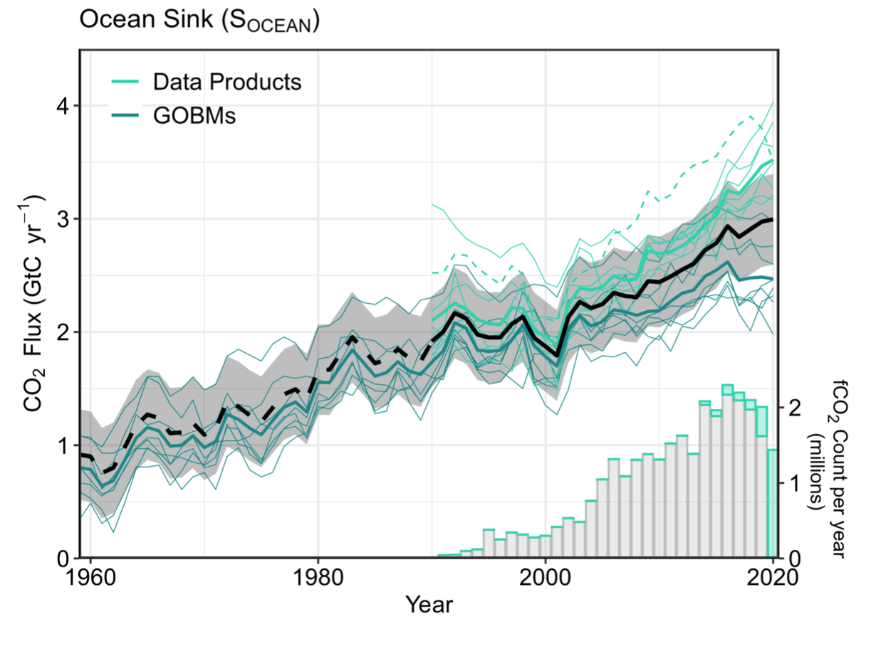
The most direct way to measure the flux of fossil fuel CO2 dissolving in the ocean is to make lots of measurements of the chemistry of the surface ocean. The rate at which CO2 dissolves into the surface ocean or evaporates from it depends on the extent of chemical disequilibrium between the air and the water: the larger the disequilibrium, the larger the rate of CO2 flux.
The CO2 of the surface ocean is wildly variable, ranging from 250 ppm in some locations and seasons up to 500 ppm in others. The atmospheric value is at 415 ppm (in 2022), varying with a seasonal cycle of 10 ppm in some places. These spatial differences mean that in some locations there is an average CO2 flux dissolving into the oceans and that in others, there is CO2 degassing. In total, there are CO2 exchange fluxes into and out of the ocean of approximately 90 Gton C per year. If, on average, there is a difference between the total CO2 fluxing in and the total CO2 fluxing out, then there is a ‘net flux’ of CO2.
The net flux of oceanic CO2 is estimated using two approaches: those that are based on global ocean biogeochemistry models and those that are based on measurements. If multiple independent approaches arrive at similar conclusions we can have more confidence in the results. Below are model- and measurement-based estimates of the ocean CO2 flux since 1960. These different approaches show an increase in CO2 net flux into the ocean, from about 1 Gton C in 1960 to a little less than 3 Gton C in 2020.
Land Uptake
As mentioned previously, Earth’s land surface is far more complex than the ocean. While many measurements have been and continue to be made of CO2 fluxes into and out of the land surface, it is a very challenging task to estimate a net flux of CO2 for all land areas.
Nearly all methods for estimating land carbon fluxes rely on some kind of land carbon model. These are mathematical computer models that keep track of the amount of carbon in the soils and on the land surface (the carbon pools) and they also model the exchange of carbon between the land and the atmosphere (the carbon fluxes). The carbon pools and fluxes depend on how the plants and soils interact and respond to the climate and to other changes on the land.
To make this more precise, let’s think about a single tree in a forest. That tree grows by taking in carbon through photosynthesis, \(\ce{CO_2 + H_2O + photons}\) \(\ce{ \rightarrow CH_2O + O_2}\), where \(\ce{CH_2O}\) represents the carbon the tree uses to make its leaves, wood, and roots. The tree can store carbon underground by growing its roots or it can store it indirectly by transferring carbon-enriched compounds to soil microbes that help the tree, such as fungi known as mycorrhizae. Above the ground, the tree stores carbon by growing its leaves and branches. The amount of carbon the tree allocates to each of these depends on the climate it experiences and the soil that it is growing in as well as the genetics of its species. The tree will grow old and die or it may be killed by beetles or burned in a forest fire.
In order to model land carbon fluxes, we have to be able to model all these fundamental processes. And not just for this one tree, but for every tree and plant in every soil and climate type on Earth. Given how complex and interconnected even a small section of forest is, you can see how much of a challenge this would be to do it for the entire global land surface. Given the complexity involved, modeling absolutely everything would be impossible, so many approximations must be made in the carbon models. The models are being constantly refined based on experiments in labs, observations of specific forests and fields, and measurements taken from satellites.
The current best land carbon models and observations indicate that the land surface is both emitting and absorbing carbon in roughly similar quantities. As we see in the figure below (Friedlingstein, et al., 2022), land use changes since the 1960s have emitted about 1-2 Gton C per year (left-most panel). There has also been absorption or a sink of about 1-4 Gton C per year (middle panel), with a large year-to-year variability. If you combine these two components (right-most panel, boxed in orange) you see that, on average, there is a current net flux of carbon into the land surface of about 2-2.5 Gton C per year, though prior to the 1970s there was a net flux of carbon out of the land surface (due to deforestation and land use changes).
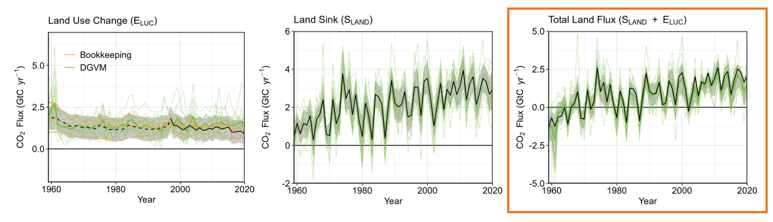
What’s causing this trend of a more positive net flux into the land since the 1980s? In the carbon cycle models it is due to primarily two effects. One is global warming’s lengthening of the growing season outside the tropics, allowing plants, especially in the coldest regions, to grow more and store more carbon. The other larger effect is a CO2 fertilization effect, which stimulates plants to grow faster or larger in a higher-CO2 atmosphere. Leaf photosynthesis takes place behind a waxy seal, with gas ports called stomata that can be actively opened and closed. The penalty for opening the stomata is the loss of water as vapor. If the CO2 concentration in the air is higher, the plants can grow without losing as much water, so they often grow more. The enzyme responsible for CO2 uptake, called rubisco, also runs more quickly at higher CO2 concentrations.
Carbon Cycle Balance
Let’s now see what the balance looks like when we put together all of the components: the increase of carbon in the atmosphere, the increasing sink of carbon into the ocean, and the increasing sink of carbon into the land.
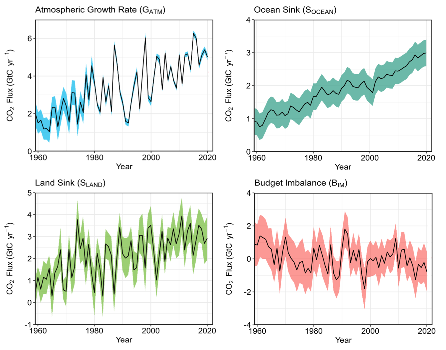
These represents our current understanding of where the carbon is going. Note that this figure also shows a ‘Budget Imbalance’ plot. This is the amount of carbon that, for each year, is not accounted for in the models and observations-based estimates of the carbon cycle; it mostly represents the amount of imperfection in our current models of the carbon fluxes of the ocean and particularly the land. You may also notice that the ‘Atmospheric Growth Rate’ has much more year-to-year variability and is not as smooth as the famous Keeling curve of CO2 from Mauna Loa in Hawaii. This is because the growth rate is a measure of the year-to-year rate of change of carbon in the atmosphere, not simply the value of carbon in the atmosphere each year like in the Keeling curve. This difference emphasizes year-to-year fluctuations in the rate of carbon entering the atmosphere. While the human emissions are fairly steady year-to-year, variability in the atmospheric growth rate is mostly driven by carbon fluxes into and out of the ocean due to a natural climate phenomenon called the El Niño-Southern Oscillation (which we will discuss in more detail in the following chapter).
The Future of the Carbon Cycle
Currently, on a time scale of decades, the carbon cycle is absorbing the blow of global warming by taking CO2 out of the atmosphere. But there are reasons to worry that the land biosphere could release more than it takes up with an intensification of warming. The concentration of organic carbon in soils is a strong function of temperature. This is because when a leaf falls into the dirt, it decomposes more quickly in warm conditions than colder ones. Generally, the rates of biological processes such as decomposition approximately double in response to 10°C of warming (up to a point, until the biomolecular machinery starts breaking down). Soil carbon levels are highest in the chilly high latitudes and very low in tropical soils, even in rain forests that are lush aboveground, because the carbon decomposes more quickly in the tropical soils.
Soil carbon concentrations could change dramatically in high latitudes where peat deposits are currently preserved from degradation by being frozen in soils called permafrosts. Peats are thought to contain hundreds of Gton C. Permafrost soils, depending on their thickness, can take centuries to melt, though they are now beginning to melt throughout the Arctic.
There is a zone near the soil surface, called the ‘active zone’, that melts in summer and refreezes in winter. This seasonally melted zone has been getting thicker over the past few decades in response to climate warming, potentially exposing more carbon in soils to degradation. Lakes also provide a pathway for degrading permafrost carbon around their boundaries, where the liquid water encounters the frozen soil. The anoxic condition of lake sediments provokes anaerobic fermentation of the carbon, producing methane as well as CO2, which reach the atmosphere in rings of bubbles around the lake periphery.Walter et al., Methane bubbling from Siberian thaw lakes as a positive feedback to cliamte warming, (2006).
Another carbon reservoir to watch out for is the methane hydrates in the ocean. A warming of the ocean sediment column could provoke these ices to melt, potentially releasing their methane into the ocean or the atmosphere. The potential of methane hydrates to alter the future climate is huge, but it will take millennia for global warming to penetrate the sediment column where most of the hydrate is. Methane hydrates therefore would probably add to global warming only in the very long term.Archer, Methane hydrate stability and anthropogenic climate change, (2007).
The Fate of Fossil Fuel CO2 in the Carbon Cycle
Although 70% of the Earth’s surface is covered by ocean, most of the volume of the ocean, the cold abyssal water, is in contact with the atmosphere only in the coldest of places and times: the high latitudes in winter. In these places there may be sea ice separating air from water and slowing the CO2 invasion of the deep sea even further. This bottleneck of getting gases into the abyss is why CO2 uptake in the deep ocean takes much longer than one would expect based on the kinetics of gas exchange alone.
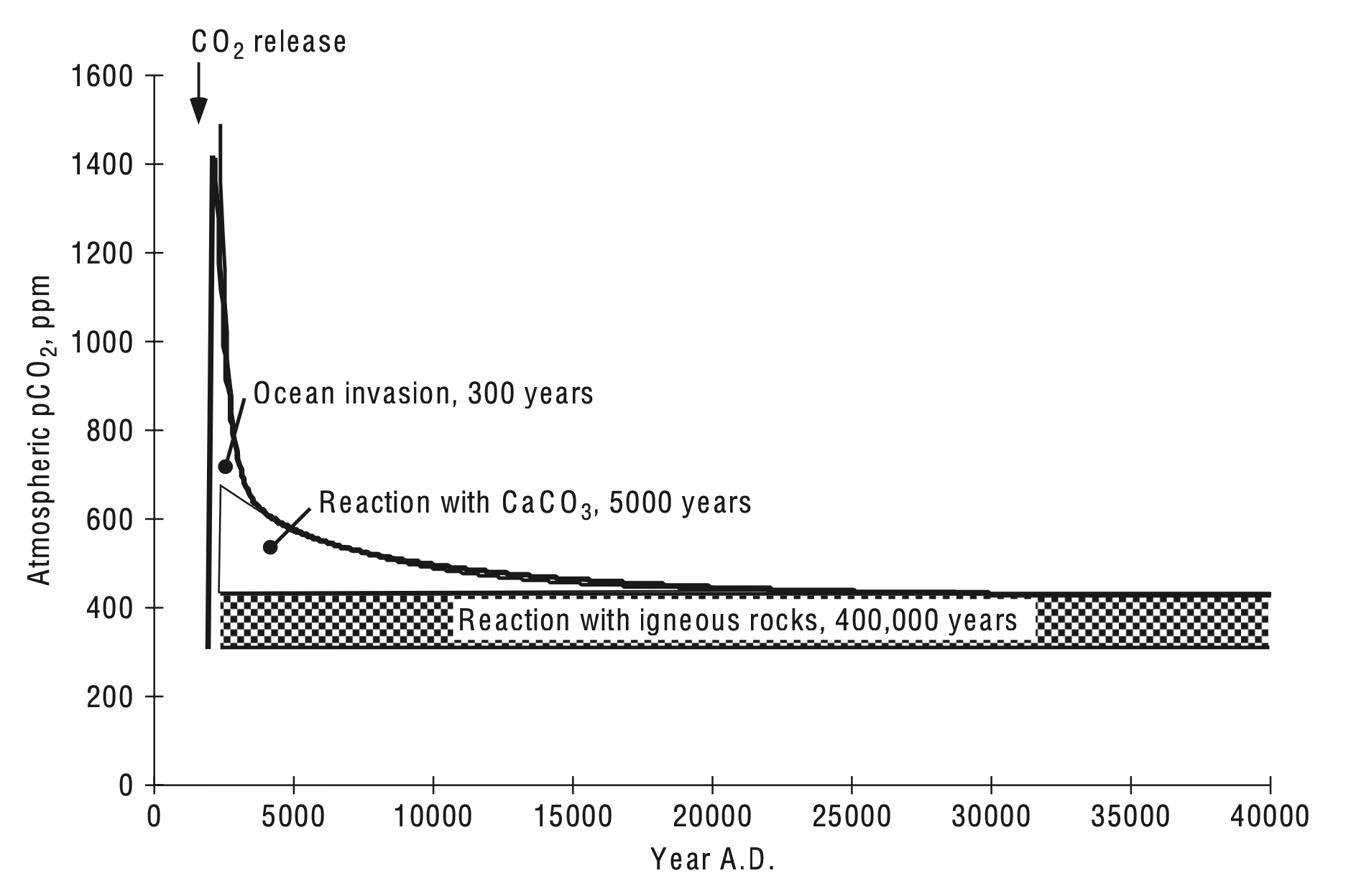
After the global warming spike of new CO2 spreads out and equilibrates between the atmosphere and the ocean, the CO2 of the atmosphere remains higher than it would have been for what carbon cycle modelers call the long tail (see figure below). The residual airborne fraction of the CO2 awaits ultimate burial by the weathering-CO2 thermostat, though this will take hundreds of thousands of years.
Over the past 10,000 years or so we have been in a relatively warm ‘interglacial’ period that was preceded by a ‘glacial’ period in which nearly all of Canada and much of Northern Europe were covered by large ice sheets. This oscillation between glacial and interglacial states has been a normal feature of Earth’s climate over the past 3 million years. These glacial cycles have been driven by cyclical changes in Earth’s orbit and tilt that change the distribution of sunlight reaching Earth. If summer sunlight isn’t strong enough to melt winter snow in certain places than that snow will stay around and slowly accumulate year after year. If this happens in the Northern Hemisphere, than a glacial climate can occur (the Southern Hemisphere doesn’t have enough land in the right places to grow significant ice sheets).
In the natural course of events, the Earth would return to a glacial climate. The glacial/interglacial cycles have taken 100,000 years overall (over the past ~1.5 million years), but the interglacial intervals have usually been short, only about 10,000 years out of those 100,000.Hays, Imbrie, and Shackleton, Variations in the Earth’s orbit: Pacemaker of the ice ages, (1976). However a few interglacials have lasted 50,000 years and Earth’s orbital features now fairly closely match those longer interglacials. So it is entirely possible that the natural future evolution of Earth’s climate would be continued warmth for the next 40,000 years followed by a gradual transition into an ice age.
The effect of the long tail of fossil fuel CO2 in the atmosphere will be to make it harder for ice sheets to form and grow in the Northern Hemisphere. The fossil fuel era will very likely make Earth skip at least one glacial period and possibly up to five, delaying the next ice age for up to 500,000 years.Archer and Ganapolski, A movable trigger: Fossil fuel CO2 and the onset of the next glaciation, (2005).
\(\Uparrow\) To the top
\(\Rightarrow\) Next chapter
\(\Leftarrow\) Table of contents