Global Climate Models
Climate Model Components
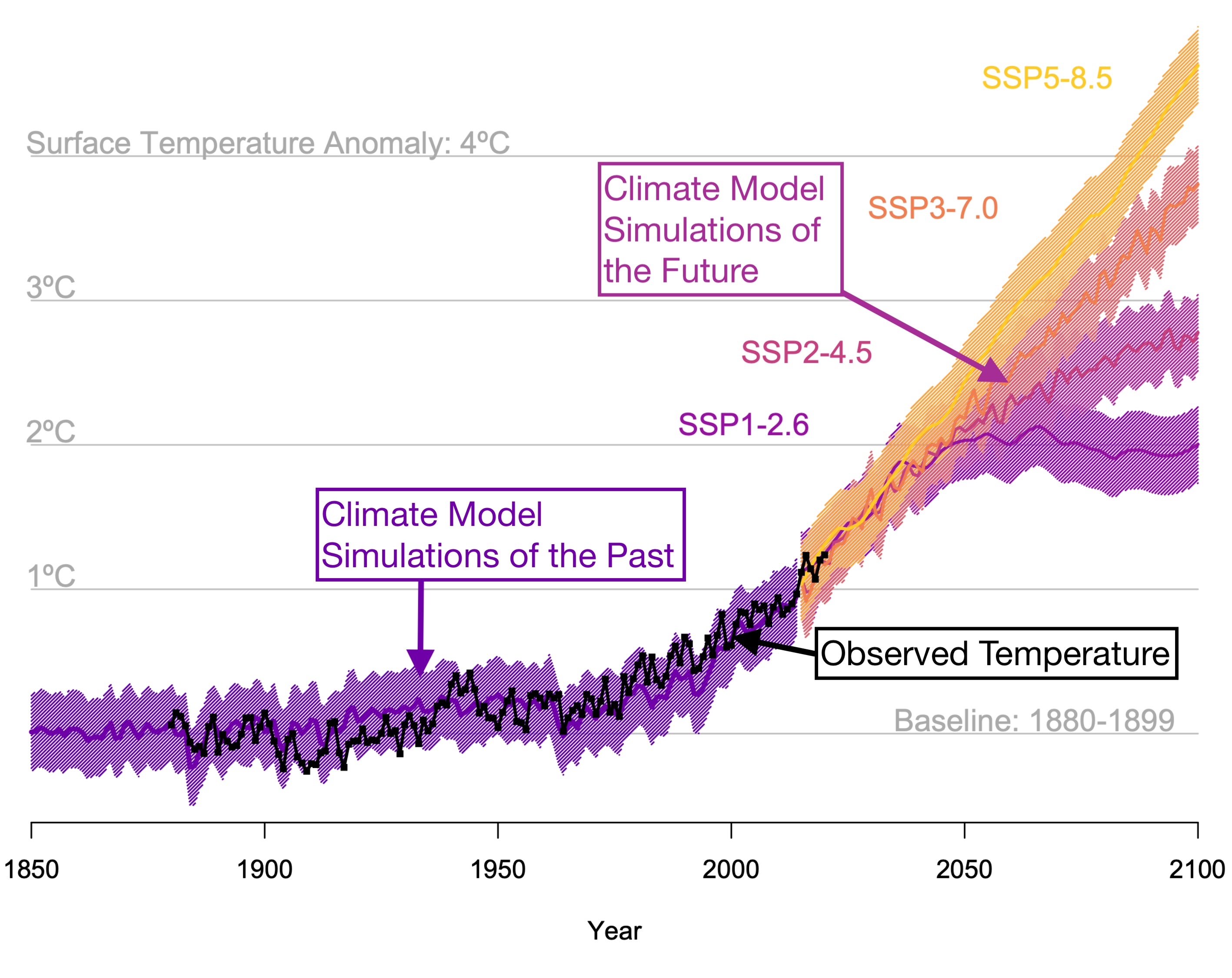
We’ve so far learned about energy balance models, carbon cycle models, and 1-D atmospheric column models. Now we’re ready to learn about the big and complex 3-D global climate models. These are the workhorse models of climate science. Most of contemporary climate science relies on these kinds of models. These are also the models that are used in nearly all of the projections of global warming, as in the figure below.
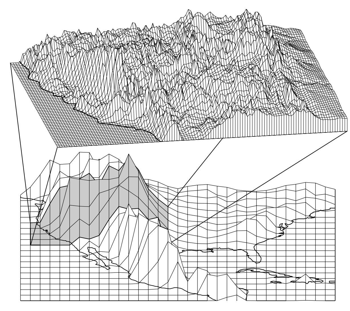
The major goal of global climate modeling is to accurately represent on a computer how the major processes of the climate system work. To do this, the atmosphere, land, and ocean have to be divided up and approximated by a finite number of grid cells. Let’s see what this looks like for some piece of ocean and land not very different from somewhere like the coast of California.
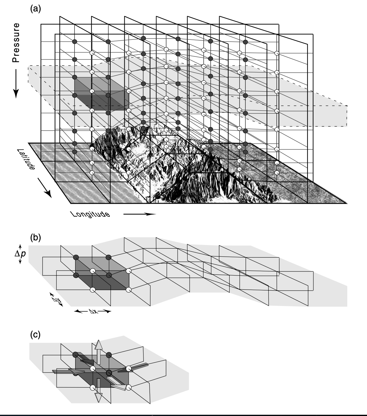
In panel (a) we see that the atmosphere overlaying the land is divided up into rectangular grid cells that follow the topography below them. In a climate model, this grid would continue globally. For each grid cell, there is a single value of each variable that the model uses, such as temperature, that represents the average over the area of the grid cell. Panel (b) shows what a level taken out of this larger grid looks like. Panel (c) indicates that climate quantities (for example, mass, energy, moisture) can move between grid cells. This kind of division of the atmosphere and ocean into grid cells means that the model can only approximate the continuous underlying motions of reality.
Some details about the grid: the vertical coordinate is a pressure coordinate modified so that it follows the topography (so it’s not actually height); the grid spacing is not constant in the vertical direction and usually not constant in the horizontal either—this is because some locations need higher vertical or horizontal resolution in order to model them well.
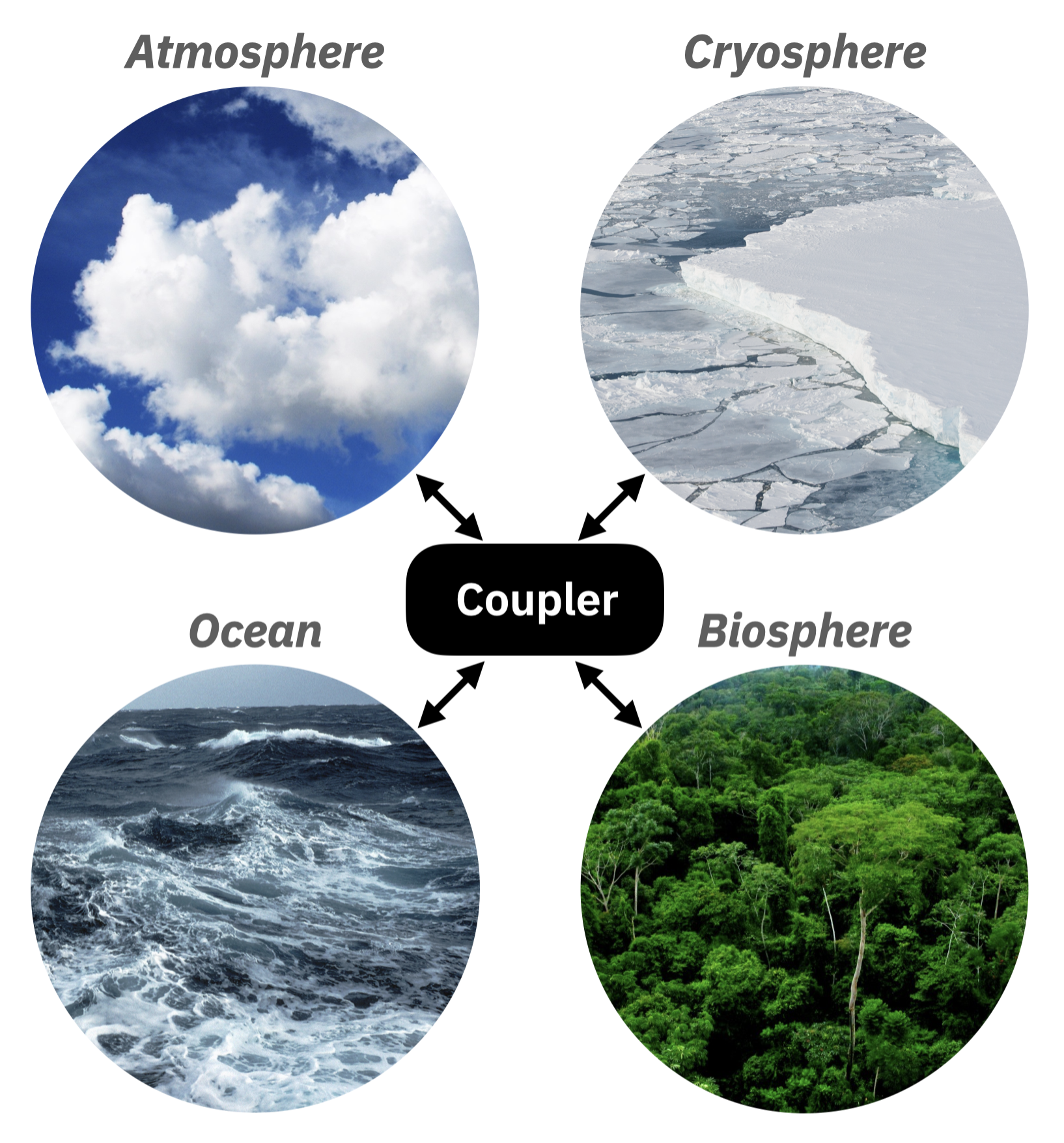
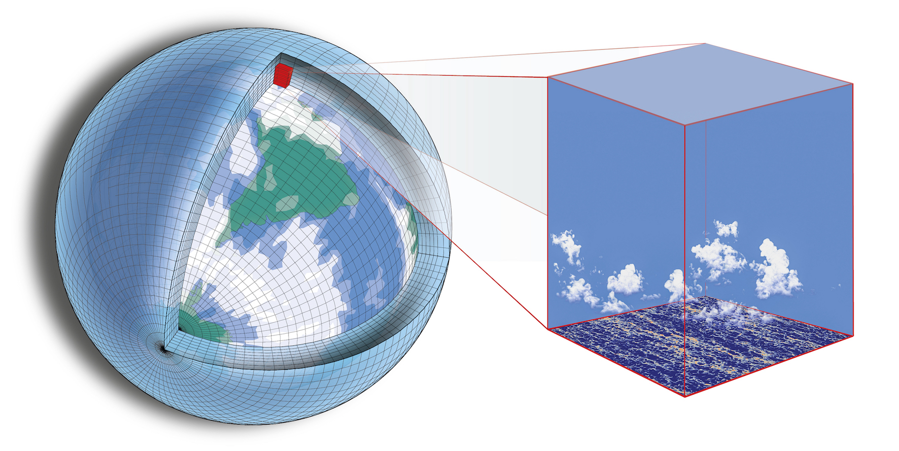
However, the grid is only the scaffolding of a climate model. More important than the scaffolding is what is built into it. A climate model is built with equations that describe the phenomena of Earth’s four climate realms: atmosphere, ocean, cryosphere, and biosphere. Each realm has its own set of equations that describe the phenomena within that realm. For example, the atmosphere has equations that describe the motions of the air, the formation of clouds, precipitation, the absorption and emission of radiation, and the chemical reactions that take place in the air. Each climate realm is connected to the other realms through a special piece of computer code called a ‘coupler’, see below.
The computer code that climate models are written in is modular: many of the components can be mixed and matched to run different kinds of simulations. For example, you can run a climate model simulation that only uses the atmosphere and its equations; or you could run a simulation that includes only the atmosphere and ocean components, and no interactive biosphere or cryosphere.
What do the equations of each realm or component look like? Written below are all the differential equations that are necessary to describe the flow of dry air (so not including water vapor or clouds), which are called the ‘Navier-Stokes equations’.
The mass continuity equation: \[ \frac{\partial \rho}{\partial t} +\nabla\cdot(\rho \vec{v})=0\] The momentum equation: \[\frac{\partial \vec{v}}{\partial t}+(\vec{v}\cdot\nabla)\vec{v} = -\frac{\nabla p}{\rho}+\nu\nabla^2\vec{v}+\mathcal{F}\] The thermodynamic equation: \[\frac{\partial \theta}{\partial t}+\vec{v}\cdot\nabla\theta=\frac{\theta}{c_pT}Q\] The equation of state: \[p = \rho\frac{R}{\overline{M}}T\]
It’s not important for our purposes here to understand these equations fully. Just notice that they include variables like velocity \(\vec{v}\), density \(\rho\), pressure \(p\), ‘potential temperature’ \(\theta\), and temperature \(T\) (among others) and that these variables are functions of time \(t\). There are a similar set of equations that describe the flow of ocean water. Such equations of motion can be derived from fundamental laws of physics and are universally used in all climate models.
There are different competing sets of equations used for phenomena like the formation of clouds, the growth of plants, and the formation of sea ice. People who develop climate models use slightly different equations for such phenomena depending on the level of detail they want to include or if they think certain equations better capture the phenomena they are working on. Many climate models have been developed over several decades and equations are added or modified over time.
How are these equations actually put to use? The equations are linked together at each grid cell and solved numerically by a computer. For an example of this, consider a simple wave of pressure as a function of longitude (\(x\)), below.
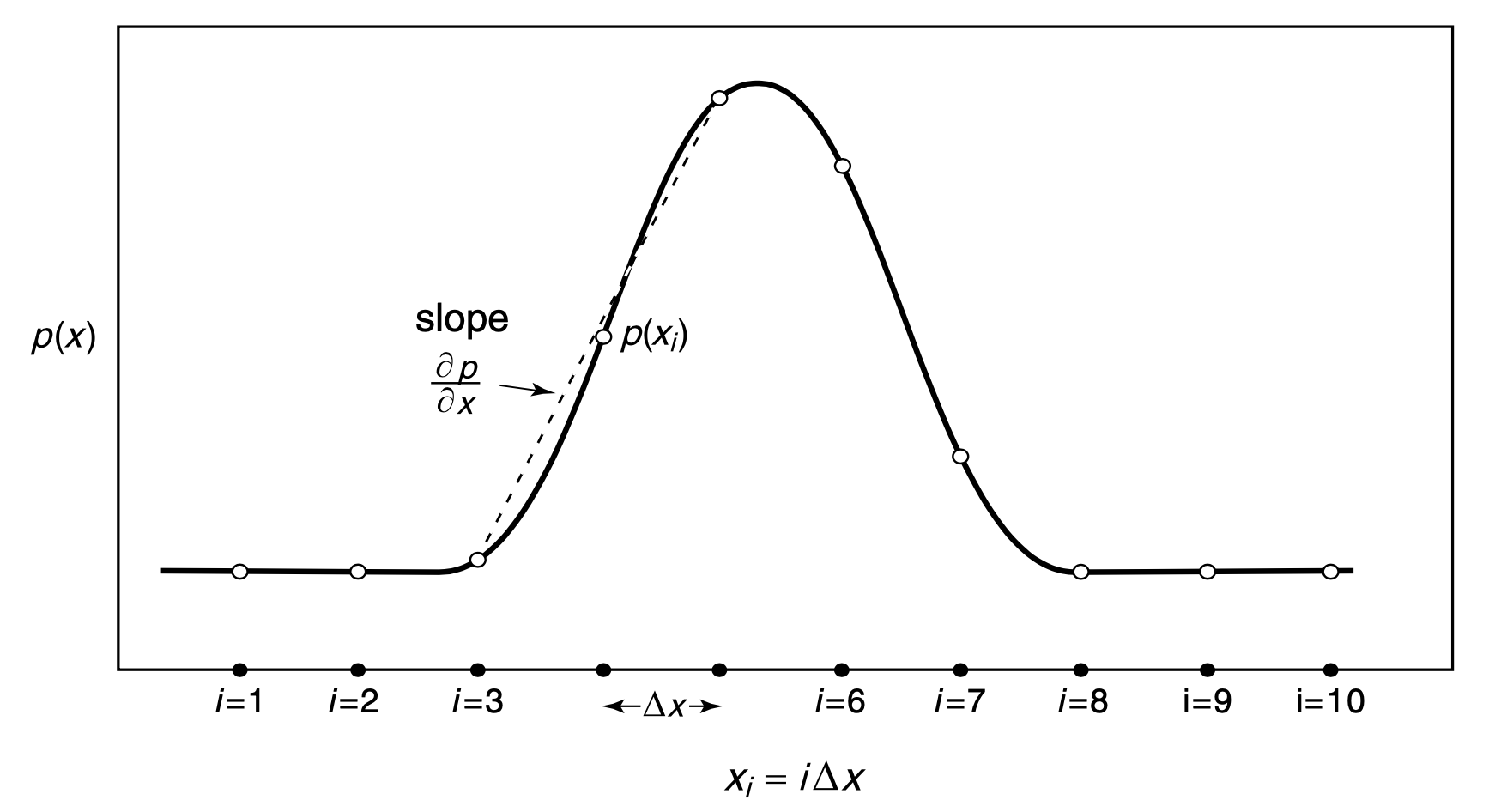
The line represents the dimension of longitude and the dots represent grid cells. The value of pressure at each grid cell is the function \(p(x)\). If we needed to compute the momentum equation, which we saw above, for this pressure field, one part of that equation is \(\nabla p\) which is equal to \(\frac{\partial p}{\partial x}\) for this one dimensional example. So we need to know \(\frac{\partial p}{\partial x}\) for all of the grid cells. This can be calculated by finding the slope at each grid cell using neighboring grid cell values. One simple way of computing the slope would be to calculate the following equation for a given grid point \(i\) and grid size \(\Delta x\), \[ \frac{\partial p}{\partial x} \approx \frac{p_{i+1}-p_{i-1}}{2\Delta x}\; .\] This approximates the pressure gradient at point \(i\). The other parts of the momentum equation, as well as other differential equations describing other variables, would be solved in a similar way. Also similar to this numerical solution technique, every climate model has a numerical method of moving the equations forward in time; this corresponds to computing the \(\frac{\partial}{\partial t}\) parts of the equations of motion listed above. Just like how the numerical solutions need to know the grid size, \(\Delta x\), so do they also need a specific ‘time step’ \(\Delta t\). Time steps are usually a few ‘model minutes’ in length.
Again, it’s not important for our purposes to understand everything about this process. What’s important to know is that there are sets of connected equations that describe how the climate realms work. These equations are solved numerically by a computer on a grid that represents Earth’s atmosphere, ocean, and land. And this numerical solution evolves in time.
The numerical output of the model from the computer, when plotted, looks just like what you might see if you could watch Earth’s weather and ocean circulation from space. Here’s an example showing only the variable of atmospheric water vapor over time.
A single simulation from a modern climate model includes hundreds of variables, each of which could be plotted and turned into a little movie like this example.
If you are curious about what the code of global climate models looks like, here are two examples you can explore on GitHub: the Community Earth System Model and the Climate Machine.
Model Resolution
As you may be able to intuitively guess from the figures above, having a smaller sized grid can significantly improve the climate model simulation. Higher resolution (smaller grid cells) allows you to resolve smaller scale processes. Relatedly, it allows you to have greater accuracy in the numerical solutions to the differential equations. The figure below compares two grid resolutions, the bottom resolution is typical of a global climate model from about 2010 while the top has a resolution that is 10 times higher.
Given that the topography looks so much more impressive at high resolution, why aren’t climate models run at even higher resolution? The main reason is computational time (which is proportional to how much it costs), which increases dramatically for high resolution. Climate models can only be run on computer clusters or ‘supercomputers’, so you have to pay for all the computational time you use on the computer system. Computational time for a simulation can be broken down into the following parts:
Computational time = (computer time per operation) × (operations per equation) × (number of equations per grid box) × (number of grid boxes) × (number of time steps per simulation)
where an ‘operation’ is, for example, a single multiplication or addition; several operations have to occur in calculating each of the terms of each of the equations for each variable in each grid box. If you increase the horizontal resolution of the model you also have to increase the vertical resolution, as well as shorten the time step of the calculations to keep things numerically accurate and stable. So increasing the resolution by, for example, a factor of 2, ends up increasing the total computational time by a factor of 16: 2 for the number of grid cells in latitude, multiplied by 2 in longitude, multiplied by 2 in the vertical, and multiplied by 2 in time, so 24=16.
If the computational time for a simulation is so long that a climate scientist cannot wait for it to be completed, the cost becomes irrelevant. To give you an idea of the time involved, if the climate model simulation is only for the atmosphere, about 20 years of climate can be simulated in about a day or two. Simulations that include both an atmosphere and ocean take about 2-3 times as long. It’s fairly common to run simulations that take a couple weeks or a month to complete. Simulations that take more than a couple months time are usually seen as impractical to carry out, though some people or organizations do run long simulations if they have a lot of time and computational resources at their command. Very few people run climate model simulations that take more than a year or so of computational time.
Model Parameterizations
What happens if there are climate processes that are much smaller than the scale of the grid cells? Such as, for example, cloud formation and convection (below)?
Important physical processes that are too small to fit on a model’s grid are included by using statistical theories called ‘parameterizations’. Parameterizations represent, for example, the effects of radiation, turbulence, and cloud formation. They are physically-based equations that predict statistics. For example, instead of trying to model individual clouds, a cloud parameterization determines the collective effect of many clouds that would live within the area of a grid cell.
Let’s look more closely at another example: the turbulent mixing of air and moisture at the boundary between the ocean and atmosphere. A schematic of this process is shown below.
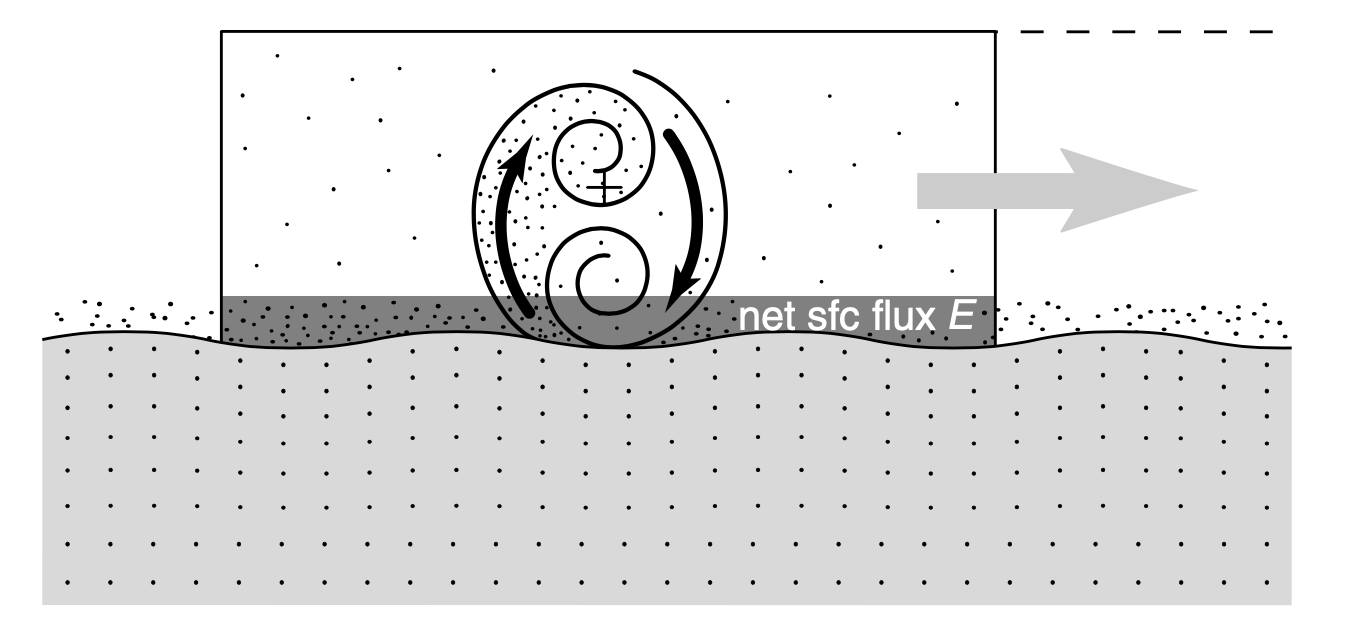
Ideally, we could model this turbulence directly, modeling all the tiny turbulent eddies of air mixing moisture into the atmosphere from the ocean. This happens on very small scales though, and is impossible to model directly. Instead we can model the flux of moisture into the atmosphere by breaking the interface down into two layers (‘level k’ and ‘level k-1’), as in the zoomed-in figure below:
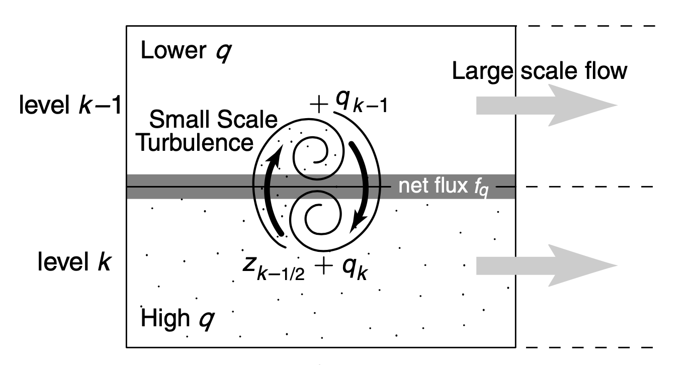
Using this two-layer model, we can then parameterize the moisture flux, \(F_q\), with a simple equation. The higher moisture air, ‘high q’, will mix with the lower moisture air, ‘lower q’, according to the difference in moisture between the two layers \[ F_q=K\frac{q_k-q_{k-1}}{\Delta z}\; ,\] where \(\Delta z\) is the height difference between the two layers and \(K\) is a numerical value that depends on the strength of the wind (the big gray arrows) and is determined by lab measurements.
Of necessity, climate models contain many parameterizations such as these. Some parameterizations are well-studied with quite a bit of confidence in their representation in models, while other parameterizations are less well understood (e.g., parameterizations of soils, plants, and clouds). Also, changing some parameterizations can have a bigger impact on climate than changing others. For example, changing cloud parameterizations tend to have bigger impacts on climate than changing soil parameterizations; the uncertainties involved in cloud parameterizations are mostly what cause the relatively large uncertainties in our estimates of cloud feedbacks.
Model Evaluation
All climate models are evaluated for their accuracy. Most major models are also continuously in development, with climate model developers seeking to improve the models in different ways. Just like in the development of computer operating systems, climate models are given version numbers as they evolve, along with short names useful for identifying them in papers, conferences, and model inter-comparison projects (for example, one of the models linked to above, the Community Earth System Model, is known as CESM). Model versions are evaluated internally by the group of developers and also evaluated externally by users of the models.
Models are evaluated in many different ways. For example, they are tested for their ability to simulate precipitation and temperature. The figure below evaluates the tropical precipitation of climate models that were a part of the Coupled Model Intercomparison Project Phase 6 (CMIP6). The top panel shows observed precipitation based on satellite measurements, the middle panel shows the average of all models in CMIP6, and the bottom panel shows the difference between the models and observations, called the ‘bias’.
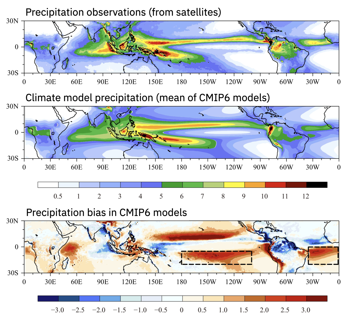
We can see that the models get the general pattern of precipitation right: it is high in a narrow band near the equator and it has a horseshoe shape over the western Pacific ocean. However the models’ precipitation tends to be too symmetric around the equator and a little too far away from the equator in the Pacific and Atlantic oceans; this shows up as the red-colored biases in the bottom panel. In particular, the bias highlighted by the dashed black lines over the Pacific and Atlantic oceans is known as the ‘double intertropical convergence zone bias’. This is one of the largest and most stubbornly persistent biases in climate models.
Another of many tests often performed is an evaluation of the models’ global mean temperature over time. The figure below shows how a very wide range of climate models do in following the observed global mean temperature from 1850 to 2020. The observed estimates of global mean temperature are in black in both panels and each model simulation is given a different colored line; the average of all models is shown with a thick red line in the top panel and in thick red and blue lines in the bottom panel.
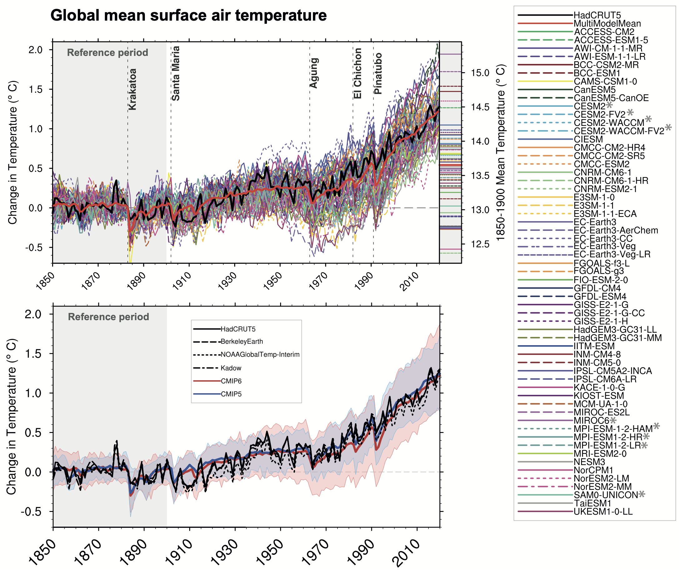
However, given that the people who develop the climate models know what the historical global mean temperature has been and that some of them test their models against it internally, the figure above isn’t entirely an independent test of the models.Hourdin et al., The Art and Science of Climate Model Tuning, (2017).
A truely independent test is to evaluate temperature projections that were made in the past. Hausfather et al., (2020) did this for every major projection of global mean temperature made by models since 1970. In the figure below they show global mean temperature projections (colored lines) versus the observed global mean temperature (black line), where the projections are plotted starting in the year after their publication.
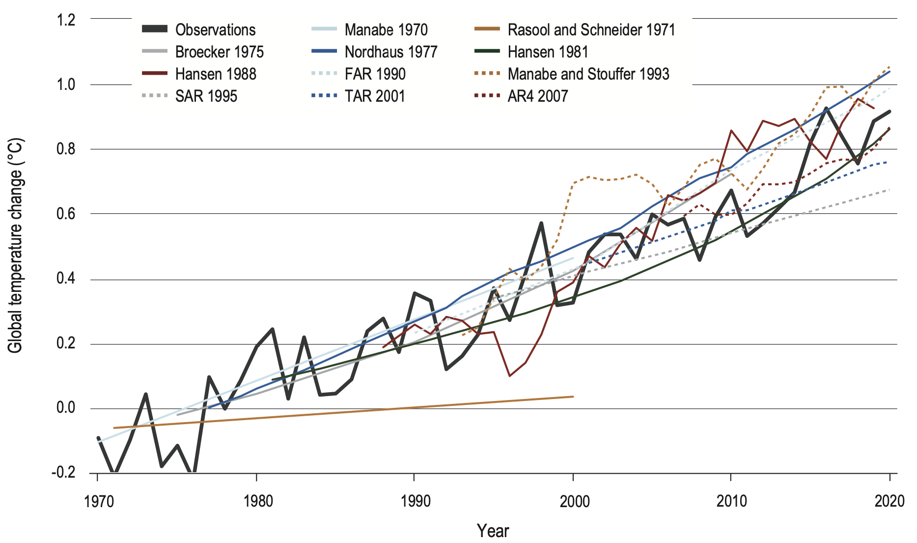
We can see that the models are generally quite accurate in their projections of global mean temperature. It’s impossible to know things like the state of ENSO in any future year or when major volcanic eruptions will occur, so the fact that they have generally been able to predict the long-term warming trend is impressive.
If your climate model has a problem, how do you fix it? Sometimes simply increasing the resolution will fix model biases. If that doesn’t work or if it’s not possible to increase the resolution, then you’ll need to modify the equations, either using fundamentally new equations or by adjusting the numerical values in the parameterizations (e.g., the value of \(K\) in the parameterization we discussed in the previous section). Adjusting the parameterizations is called model ‘tuning’ and it is necessary for any statistical or complex model in any field of science. The size and complexity of climate models means that there are many parameterizations that could be tuned, but in practice a relatively small subset are usually adjusted. The most frequently tuned parameterizations are those dealing with clouds. The values are adjusted within the uncertainty ranges of the parameter values and the results of the tuning are evaluated against a wide range of observed climate quantities.Hourdin et al., The Art and Science of Climate Model Tuning, (2017).
Climate Model Uses
Climate models are used for understanding a huge variety of climate-related phenomena, not just those directly connected to global warming. Scientists use climate models to understand things such as: the circulation of the atmosphere and ocean, the behavior of ice sheets, the nature of chemical reactions in the atmosphere and ocean, the interaction of plants with climate, the character of climates in the geologic past, and what climates might be like on planets and moons in our solar system or elsewhere in our galaxy.
Related to global warming, climate models are very useful for understanding the causes of global warming as well as its impacts. Let’s walk through an analysis using climate models that attributes observed climate changes to either human activities or natural factors. The figure below shows the global mean temperature from thermometer observations (solid black line) along with many climate model simulations that were run from the years 1850 to 2020 using different estimated radiative forcings.
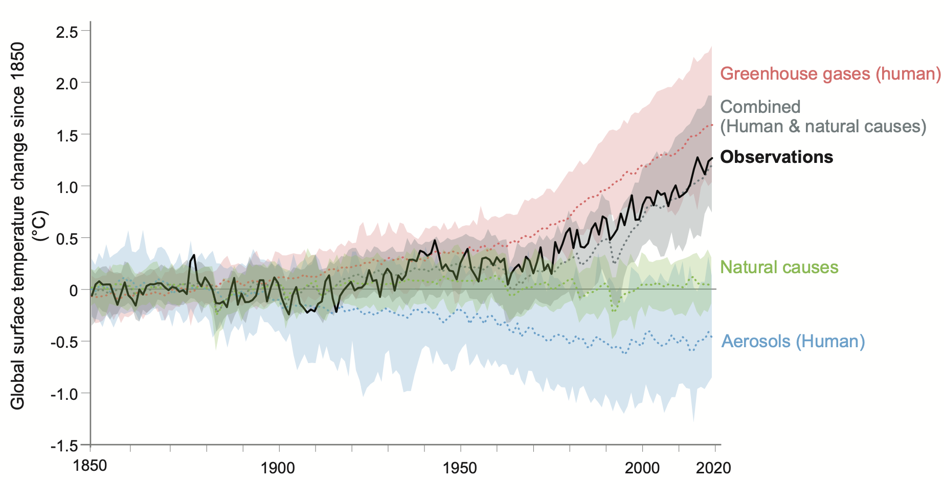
The simulations were run as an experiment testing the influence of only one particular kind of radiative forcing at a time (colors) and then all radiative forcings together (gray). The red ‘Greenhouse gases’ simulations only included greenhouse gases; the green ‘Natural causes’ simulations included only variability related to ENSO and the radiative forcings from solar variability and volcanic eruptions; and the blue ‘Aerosols’ simulations included only human emissions of soot and pollution, etc. We can see that only greenhouse gases can explain the global warming trend. But human causes alone are not enough to explain much of the year-to-year variability, which we’ve learned is caused mostly by ENSO and major volcanic eruptions. Combined, both human and natural causes can best explain the observed historical temperature variability.
There are many projected impacts of global warming and the next chapter will discuss some of the major projections and risks. Climate model simulations are particularly useful for projections because they’re really our only way to quantitatively predict what may occur in the future. But because we don’t know how humans will act in the future, climate modelers use a range of possible futures, each with its own storyline. These range from scenarios with very high greenhouse gas emissions to scenarios where emissions are rapidly reduced followed by net-negative emissions. The figure below shows how these different projections of global mean temperature and greenhouse gas emissions compare to what they have been over the past 2000 years.
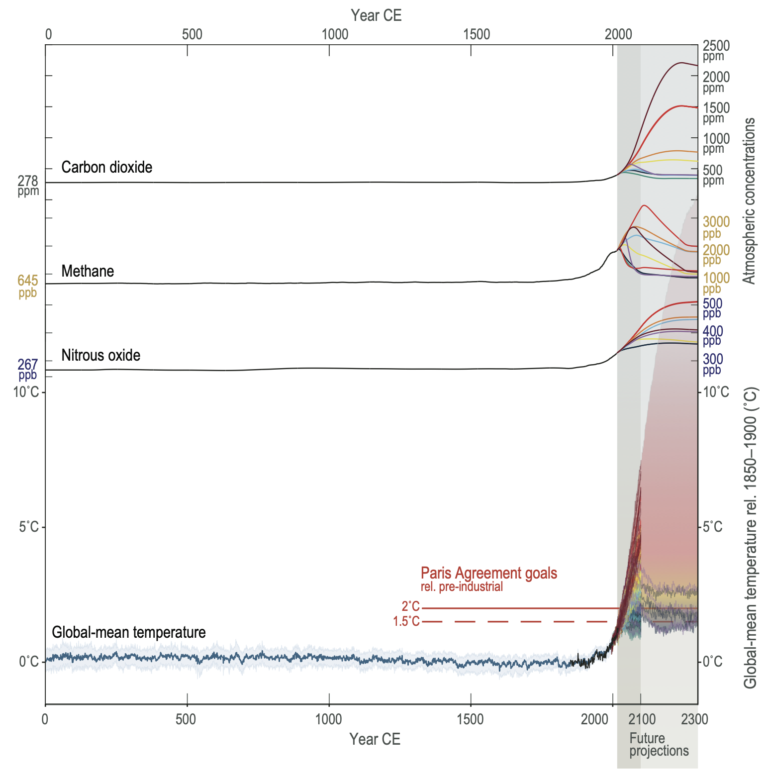
The blue global mean temperature line is based on paleoclimate proxy data (like the rings of trees), and there are model projections plotted here that go out to 2100 and some that go out to 2300. The red projections correspond to scenarios where we burn as many of the fossil fuels as we can while the blue and purple projections are scenarios where we take a lot of action to reduce fossil fuel emissions. Perhaps the future will turn out to be somewhere in the middle of these extremes? We’ll discuss these projections in much greater detail in the last two chapters. For now let’s just notice one big idea from this figure: the future is up to us. Our actions will determine whether the world will remain about the same as it is now or if it will become far warmer.
\(\Uparrow\) To the top
\(\Rightarrow\) Next chapter
\(\Leftarrow\) Table of contents