Science of the Greenhouse Effect
Energy Balance Model of Earth’s Greenhouse Effect
In the last chapter we derived an energy balance equation for a planet without an atmosphere, \[\frac{S}{4}(1-\alpha) = \sigma T^4 \; . \tag{1}\] Though by neglecting an atmosphere this equation gave us a global mean temperature that was far too cold (254 K) compared to Earth’s actual temperature (288 K). Let’s revise the energy balance model to add in an atmosphere and a greenhouse effect. This section follows the modeling approach in Chapter 1 of Vallis, Climate and the Oceans, (2011). For this revised mathematical model we’ll assume the following: (1) The atmosphere is completely transparent to solar radiation; (2) The atmosphere is opaque to infrared radiation so that it absorbs infrared radiation and acts like a blackbody; (3) The Earth’s surface and it’s atmospheric layer have a single average temperature, each denoted by \(T_s\) and \(T_a\). Assumption (1) is actually fairly realistic. Assumption (2) is somewhat realistic and assumption (3) is just so that we can keep things simple.
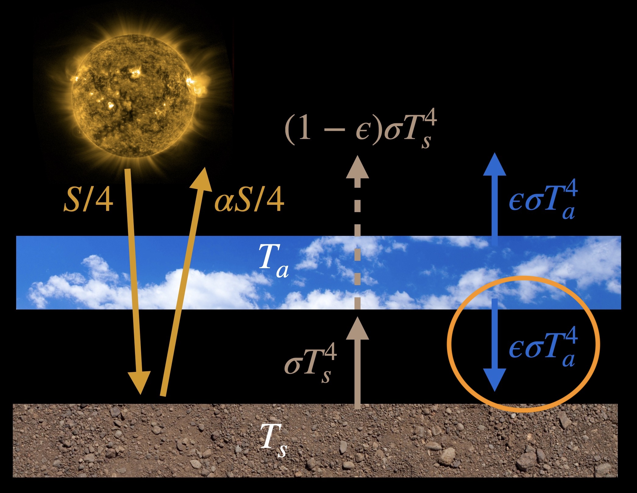
Here’s an illustration of this model with equations showing where the energy comes from and where it is going:
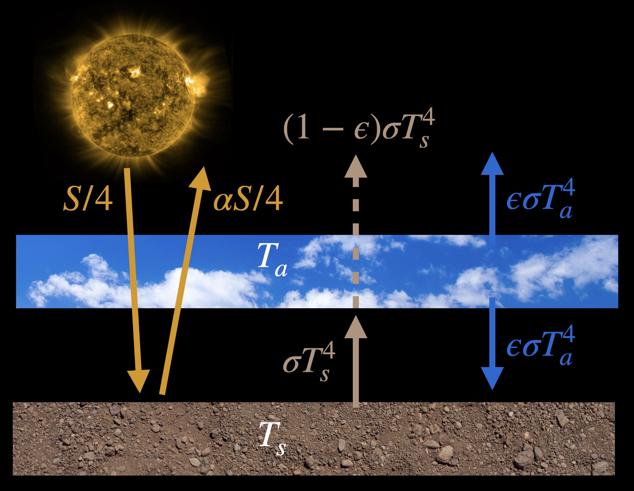
The parameter \(\epsilon\), called the emissivity or the absorptivity, determines what fraction of infrared radiation coming from the surface is absorbed by the atmosphere.
To derive the equations for this model we’ll need to balance energy going into and out of each component. So we balance all the radiation arrows going into and out of the surface and all the radiation arrows going into and out of an imaginary line that we’ll draw at the ‘top of the atmosphere’, which is actually above the atmospheric layer here. And let’s initially assume that \(\epsilon=1\), that is, the atmosphere is a perfect blackbody and absorbs all the surface infrared radiation. Here’s the energy balance equation for the surface, \[\frac{S}{4} + \sigma T^4_a = \alpha\frac{S}{4}+\sigma T^4_s \; ,\] and moving solar radiation over to one side, \[\frac{S}{4}(1-\alpha) + \sigma T^4_a = \sigma T^4_s \; . \tag{2} \] The equation for the imaginary ‘top of the atmosphere’, with \(\epsilon=1\), is \[\frac{S}{4} = \alpha\frac{S}{4}+\sigma T^4_a \; ,\] or equivalently \[\frac{S}{4}(1-\alpha) = \sigma T^4_a \; . \tag{3}\]
Notice that equation (3) is the same energy balance equation as our first model, equation (1). So our initial equation actually applies best to the energy balance at the top of the atmosphere.
We can now solve equations (2) and (3) for \(T_a\) and \(T_s\) to get \[T_a=\left[\frac{S}{4\sigma}(1-\alpha)\right]^{1/4} \; ,\] \[T_s=\left[\frac{S}{2\sigma}(1-\alpha)\right]^{1/4} \; .\]
Using \(S=1361 \text{W}/\text{m}^2\) and \(\alpha = 0.31\) we get \(T_a=254\, \text{K}\) and \(T_s=302\, \text{K}\). Our atmospheric temperature is the same as before but the surface temperature is now warmer: we now have a greenhouse effect! Though \(302\, \text{K}\) is too warm compared to the actual average temperature of the Earth \(288\, \text{K}\). The surface temperature is too warm because we are assuming with \(\epsilon=1\) that the Earth’s atmosphere is a perfect blackbody, absorbing all the infrared radiation that hits it. In fact we know from observations that some of the infrared radiation emitted by the surface escapes to space, so let’s account for that.
Instead of assuming that the atmosphere absorbs all the infrared radiation emitted by the ground, let’s assume that it absorbs just a fraction, \(\epsilon\), of it, where \(0 \lt \epsilon \lt 1\). Thus looking at the model figure above we see that an amount \((1-\epsilon)\sigma T^4_s\) of surface radiation escapes to space. Similarly, we also assume that the atmosphere only emits an \(\epsilon\) fraction of the amount it would as a perfect blackbody. In all other ways the model is the same as above. If we follow the same process of balancing energy in with energy out for the surface and the top of the atmosphere (or planet as a whole) we get the following equations:
\[\frac{S}{4}+\epsilon\sigma T^4_a = \alpha\frac{S}{4}+\sigma T^4_s \; , \] \[\frac{S}{4}=\alpha\frac{S}{4} + (1-\epsilon)\sigma T^4_s + \epsilon\sigma T^4_a\; . \] Solving these two equations for \(T_s\) we obtain \[T_s=\left[\frac{S(1-\alpha)}{2\sigma(2-\epsilon)}\right]^{1/4} \; . \tag{4}\]
If \(\epsilon = 1\), we recover our most recent greenhouse effect result with \(T_s = 302 \text{K}\). If \(\epsilon = 0\), then the atmosphere has no radiative effect and, as in equation (1), we obtain \(T_s = 255 \text{K}\). The real atmosphere is somewhere between these two extremes, and for \(\epsilon = 0.8\), approximately similar to observations, we find \(T_s = 288 \text{K}\). The real emissivity on Earth actually varies by location and to model Earth more accurately we would want spatial details and even more layers in our model atmosphere, but for such a simple model it does remarkably well. Global warming is analogous to increasing Earth’s emissivity in this model: by adding more greenhouse gases to the atmosphere we increase the amount of infrared radiation the atmosphere absorbs.
Physics of Radiation Absorption and Emission
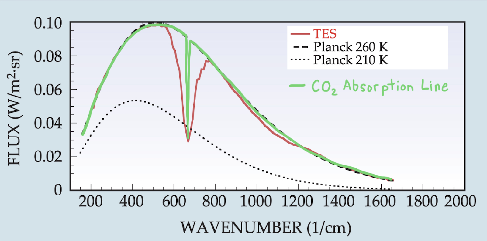
So far we’ve used the physics of blackbody radiation to explain and model the greenhouse effect. Insofar as the atmosphere behaves as a blackbody with a smooth Planck emission spectrum, this level of description is enough. But the real atmosphere is more complicated, with big gaps missing in the distribution of radiation emitted to space (known as its emission spectrum). To illustrate this, let’s first look at the atmosphere of Mars. Mars’ atmosphere is 95% CO2 and nearly all of the remaining gases do not really absorb much radiation at all. Mars is therefore a relatively simple atmosphere in which to see radiative effects. The figure below shows how the emission spectrum of Mars (red line) compares to two Planck blackbody emission spectra shown for reference (black dashed lines):
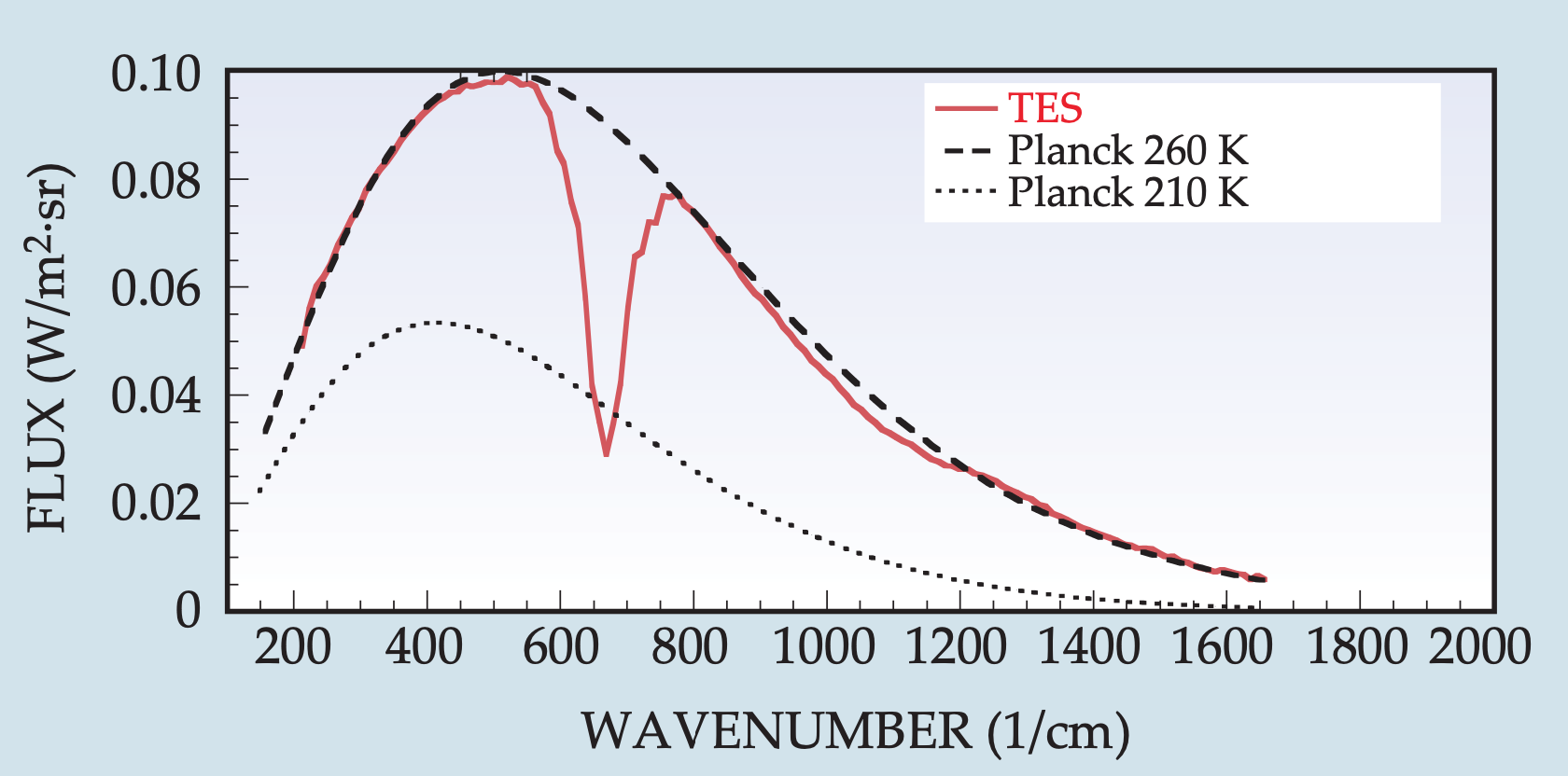
We can see that compared to the emission spectrum of a perfect blackbody, Mars is missing a big chunk of its emission centered at 667 \(\text{cm}^{-1}\) (corresponding to a wavelength of 15 \(\mu\text{m}\)). Because of Mars’ simple atmosphere we know this has to be due to CO2 absorbing radiation. So the Sun is shining on the surface of Mars, which we know from observations is then emitting radiation like an almost perfect blackbody. But then as that radiation tries to escape to space, a big chunk is absorbed by CO2 and is re-emitted back down to the surface. Much of this re-emitted radiation will be absorbed within the surface and atmosphere of Mars, warming the planet and giving it a small greenhouse effect. This process is somewhat different than changing the bulk emissivity in our one-layer energy balance model; changing \(\epsilon\) is like shifting the whole Planck emission spectrum instead of absorbing a chunk of the spectrum like what actually happens.
Let’s look now at the more complex emission spectrum of Earth (satellite observations in red, a complex atmospheric radiation model in blue):

Like Mars, Earth is missing a chunk of its spectrum centered at 667 \(\text{cm}^{-1}\) due to CO2. Yet Earth is missing additional chunks, relative to the Planck spectrum at 285 K, with the primary atmospheric gases at fault labeled at the top of the graph (H2O, CO2, O3). There are also two broad regions in which there is relatively little absorption and the emission spectrum follows the 285 K Planck distribution fairly well. These regions span approximately 800-1000 \(\text{cm}^{-1}\) and 1100-1250 \(\text{cm}^{-1}\) and are called ‘atmospheric windows’ because the atmosphere is essentially transparent to infrared radiation in these wavenumber ranges.
How physically are gases like CO2 and \(\text{O}_3\) removing chunks of the emission spectrum? Let’s start by looking at individual atoms, using the simple element Helium in particular. Like all atoms Helium is composed of a nucleus and electrons that orbit the nucleus. It looks something like this:
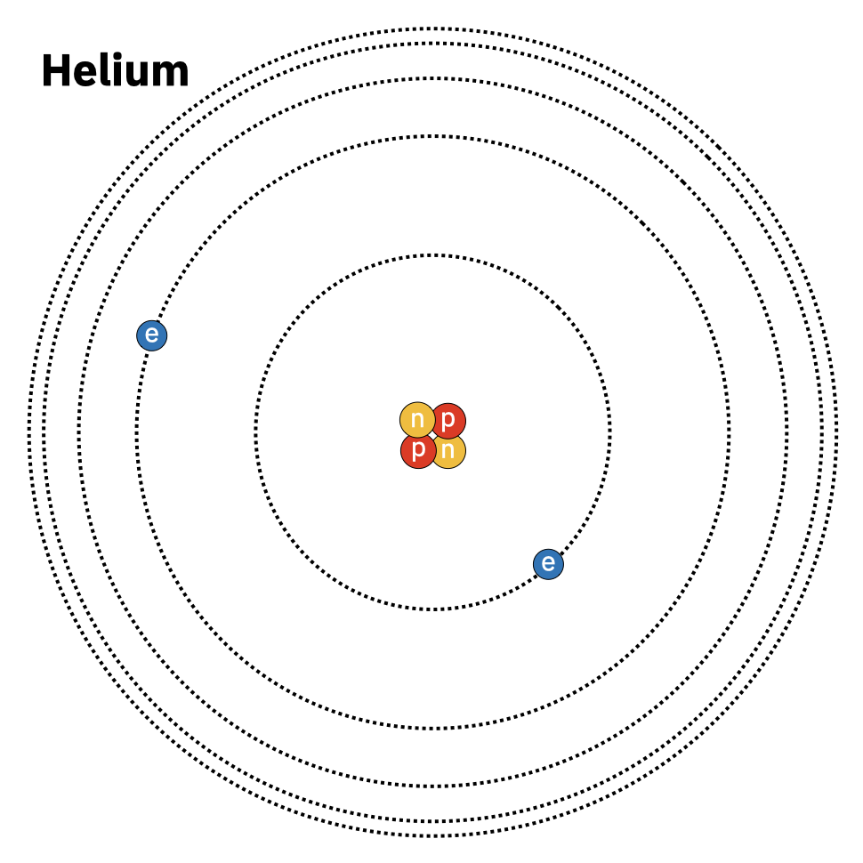
The nucleus of Helium contains two protons and two neutrons, which account for nearly all the mass of the atom. The two electrons of Helium are moving around the nucleus in very particular orbits. It turns out, due to the laws of quantum mechanics, that there are only a few specific orbits allowed around the atom. The orbits closer in are lower energy levels and orbits further out are higher energy levels. I have to note that I’ve drawn Helium using what’s called the ‘Bohr model’ of the atom that looks like planets orbiting a star. In truth the electrons aren’t hard balls that zip around the nucleus but are more like a wavy cloud that shifts its density around the nucleus. Yet the Bohr model is useful for illustrating how photons are absorbed and emitted by atoms:
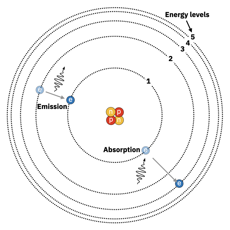
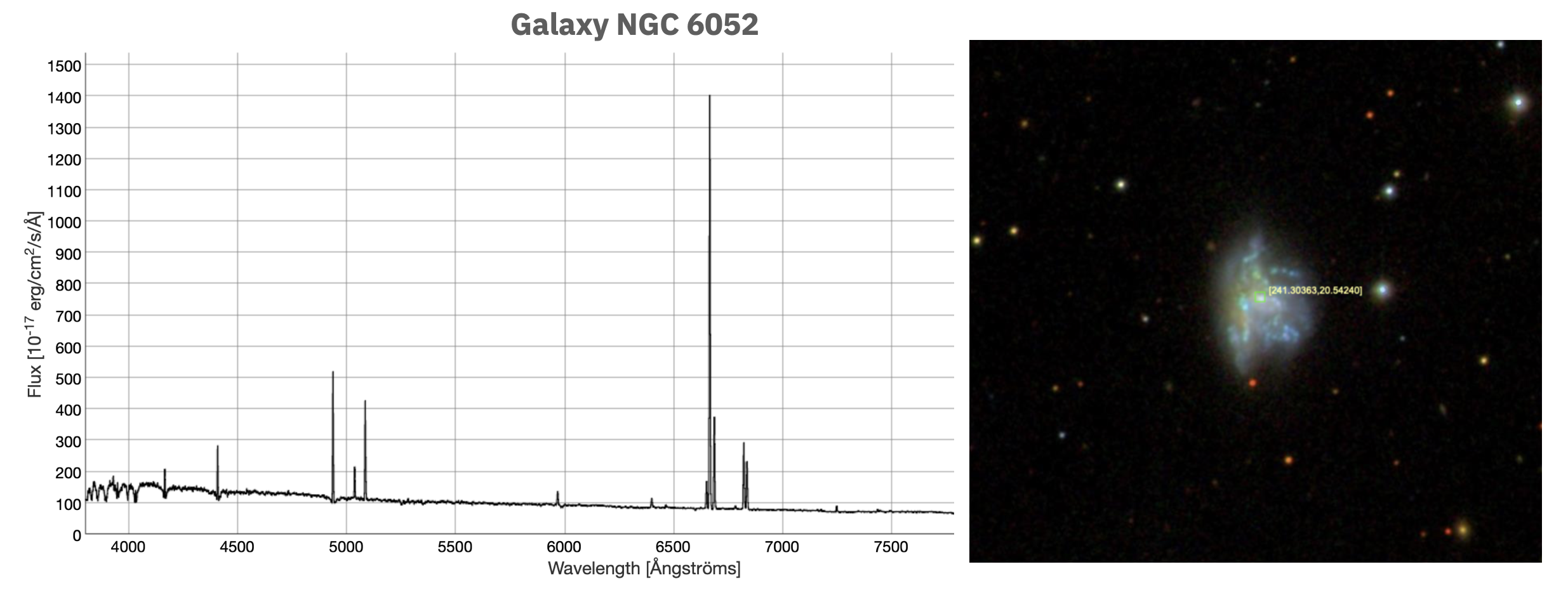
We learned in the previous chapter that photons are packets of energy, the amount of which is determined by the frequency, \(\nu\), of the photon \(E=h\nu\). As we see in this above figure, if an electron absorbs a photon, the energy of the photon goes into jumping the electron into a higher energy level. A little strangely, the photon energy must be precisely* *Technically not absolutely precisely. Very small differences are allowed via the laws of quantum mechanics. the energy required for the jump. This implies that only photons of relatively few specific frequencies can be absorbed by a given atom; for this jump from energy level 1 to energy level 3 in the illustration, the energy required is \(E_3-E_1=h\nu_{1\rightarrow 3}\), where \(\nu_{1\rightarrow 3}\) is the specific frequency of the photon for this situation. It’s a very similar process for photon emission: electrons move from a high energy level to a lower energy level by emitting a photon of precisely the right frequency to make up the difference in energy for the jump. Electrons prefer to be in the lowest energy level they can and will spontaneously emit photons to get there. But once an electron is in the lowest energy level surrounding the nucleus, an electron can’t emit photons anymore. Notice also from the figure that electrons can jump up or down multiple energy levels as long as the right frequency of photon is involved. Note: Quantum mechanics does technically forbid very specific kinds of photon energy level transitions, but that’s not important for our purposes here. This whole process explains why we only saw a few radiation peaks in the emission spectrum of galaxy NGC 6052 in the previous chapter (reproduced below); the emission was coming from primarily Hydrogen and Helium gases (what galaxies are primarily made of) and they can only emit particular frequencies of photons.
Besides absorption and emission of photons within individual atoms, it’s also possible for groups of atoms, called molecules, to collectively absorb and emit photons. The large majority of atmospheric gases are groups of either two or three atoms, called diatomic molecules and triatomic molecules; examples include \(\text{O}_2\), diatomic, and CO2, triatomic. Like in atoms, the electrons in molecules shift around in a wavy cloud of negative charge. The laws of physics dictate that in order for this electron cloud to absorb and emit photons its charge distribution needs change speed or change direction (moving at a constant speed will do nothing). A molecule’s electron cloud can do this if the molecule as a whole rotates or vibrates in particular ways. Let’s look at some examples for diatomic and triatomic molecules:
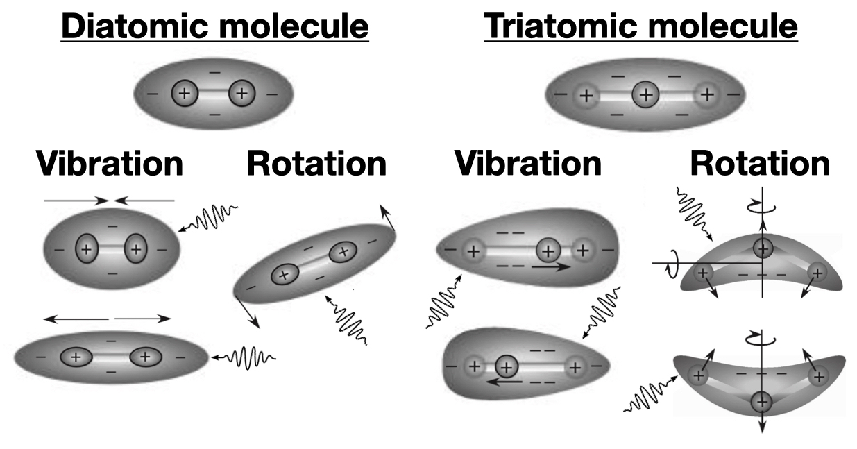
The top row of both the diatomic and triatomic molecules is the lowest energy state of the molecules. This is similar to when electrons are in the lowest energy level in an atom. The rows below that show the molecules absorbing photons and subsequently vibrating and rotating. Molecules are also able to vibrate and rotate at the same time, illustrated with the bending vibration in the triatomic ‘rotation’ column of the figure.
Just like for atoms, a molecule absorbs a photon to go from a low energy state to a higher energy state and emits a photon to go from a high energy state to a lower energy state. For example, a triatomic molecule will emit a photon when it goes from a stretched-out high energy state to its lowest energy state (the state shown in the top row of the figure above). And also just like for atomic emission and absorption, the photon energy needs to be just the right amount for the molecule to vibrate or rotate in one of the limited number of ways that it is able to. For example, CO2 is a triatomic molecule and its bending mode, illustrated in the ‘rotation’ column in the figure, absorbs photons with a wavelength of 15 \(\mu \text{m}\), corresponding to the missing emission chunk centered on the 667 \(\text{cm}^{-1}\) wavenumber in the spectra of Mars and Earth that we saw previously; this particular bending of CO2 is therefore responsible for almost the entire greenhouse effect on Mars and a large portion of the greenhouse effect on Earth (approximately 20%).
The bending vibration mode of CO2 is so important because it just so happens to overlap with an important section of the blackbody emission spectrum of Earth. CO2 has many atomic and molecular absorption energies, but just one of them really matters for Earth’s greenhouse effect. 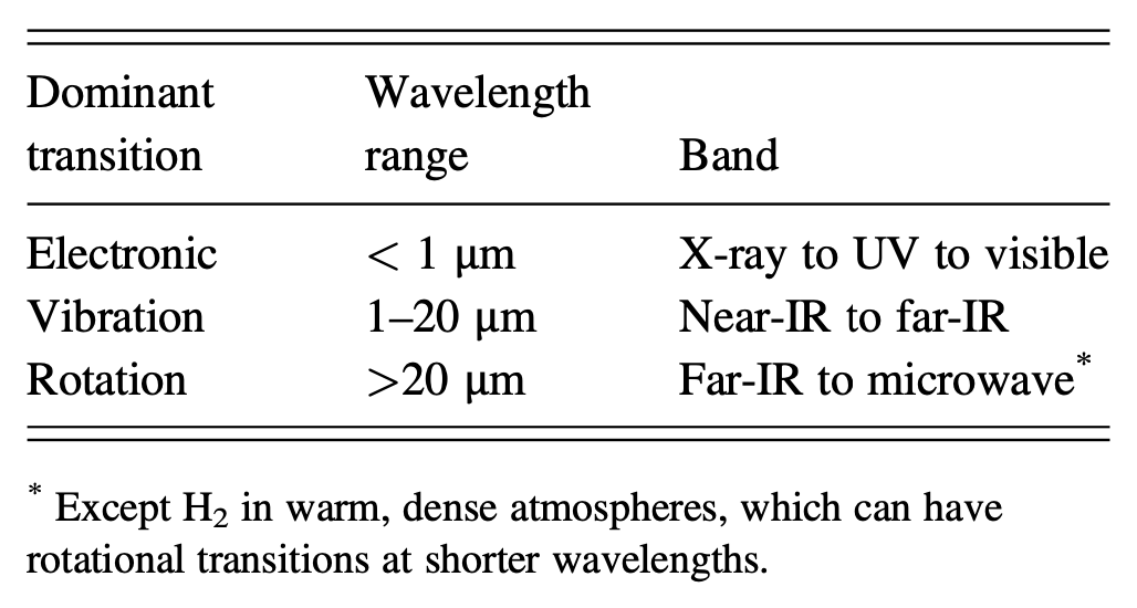 Types of radiation absorbed by atomic or molecular transition type. An ‘electronic’ transition is equivalent to what I’ve been calling in this chapter ‘atomic’. Increasing wavelength corresponds to decreasing energy, according to the equation for photon energy \(E=hc/\lambda\). IR is short for ‘infrared’. Catling and Kasting, Atmospheric Evolution on Inhabited and Lifeless Worlds, (2017). Whether a gas is radiatively important or not is entirely determined by this overlap between a gas’ photon absorption energies and the spectrum of photon energy emitted by the planet. In general, atomic absorption requires the highest energy photons, followed by molecular vibration, followed by molecular rotation with the lowest required energies, see side table. Since Earth, as well as many other planets, emits primarily infrared radiation, it turns out that vibrational and rotational modes of atmospheric gases dominate the greenhouse effect, see side table.
One feature of the emission spectra we saw of Mars and Earth that we have not explained yet is why the missing emission chunks are so wide? All the explanations given so far for photon absorption have said that the physics of atoms and molecules allows only particular, individual electron energy states to exist. If atoms and molecules can only absorb photons of a few particular energies or frequencies, why do we see wide bands in the emission spectra instead of narrow lines? Why doesn’t the emission spectrum of Mars look like the green line I’ve drawn over the top of this figure?
Photon absorption is broadened from narrow lines into wide bands due to two processes: Doppler broadening and pressure (or collision) broadening. Doppler broadening happens when gas molecules move relative to the source of radiation. Like the changing sound of a fast-moving car that passes us, the sound of the car has a higher pitch or frequency as it approaches us and then a lower pitch or frequency as it moves away. Similarly, the frequency of radiation that hits a moving molecule will be ‘Doppler shifted’: if the molecule is moving toward a radiation source, the frequency and energy of photon it can absorb will be increased slightly; and if it’s moving away from the radiation source, the frequency and energy of the photon it can absorb will be decreased. Pressure (or collision) broadening happens when collisions between molecules happen at the same time as photon absorption and some of the energy of the collision adds to or subtracts from the energy required for the photon absorption.
The shape of the broadening from these two processes that we see in emission spectra (as in our Mars example above) follow what are called the Doppler and Lorentz line shapes:
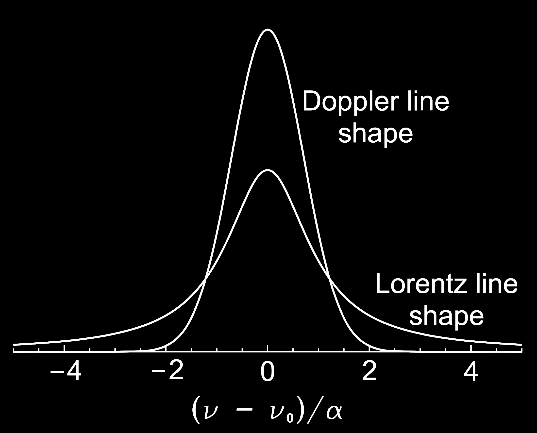
In general, pressure broadening is the dominant broadening process in the troposphere and lower stratosphere. Doppler broadening dominates in the upper stratosphere and above Catling and Kasting, Atmospheric Evolution on Inhabited and Lifeless Worlds, (2017). because the dramatically reduced pressure at those heights means that collisions do not happen enough for pressure broadening to be as important.
Doppler and pressure broadening are absolutely essential for the greenhouse effect. Without these processes only a tiny fraction of the radiation energy could be absorbed by the atmosphere. Therefore the greenhouse effect wouldn’t exist at all Catling and Kasting, Atmospheric Evolution on Inhabited and Lifeless Worlds, (2017). and Earth would be a frozen and uninhabitable \(T=254\, \text{K} \approx -20 ^{\circ}\text{C}\), as we calculated.
If we go back to the emission spectrum of Earth we saw above and we compare the radiation absorption due to different gases, we can see a big difference between the effects of \(\text{H}_2\text{O}\) and CO2 or \(\text{O}_3\):
CO2 and \(\text{O}_3\) are absorbing radiation in lines broadened into bands, while \(\text{H}_2\text{O}\) is absorbing radiation over wide ranges of the spectrum. This kind of absorption is called ‘continuum absorption’ and is due to \(\text{H}_2\text{O}\) being a particularly good absorber of many kinds of infrared radiation; this is due to \(\text{H}_2\text{O}\)’s molecular shape and its many vibrational and rotational modes. The ability of \(\text{H}_2\text{O}\) to absorb radiation across wide continuums is what makes it the most important greenhouse gas in Earth’s atmosphere. Water vapor alone is responsible for approximately 50% of the greenhouse effect and water-based clouds another 25%. Schmidt et al., The attribution of the present-day total greenhouse effect, 2010. Such large values for \(\text{H}_2\text{O}\) may cause you to wonder why we focus so much attention on CO2, which contributes approximately 20% of the greenhouse effect. As we will discuss in Chapter 8, it is CO2 that is largely responsible for the amount of \(\text{H}_2\text{O}\) in the atmosphere, thus CO2 is actually the gas that is radiatively in charge even though \(\text{H}_2\text{O}\) has a much bigger greenhouse effect.
Another fundamental question is why do we even have gaps in the emission spectra of planets at all? If an atmosphere can emit photons at the same energies that it absorbs them, why can’t the atmosphere just pass along the photons to outer space? Part of the answer has to do with the direction of emission: photon emission in a gas occurs in random directions (as shown in the illustrations), so it’s not possible to just convey the photons directly out to space. The other part of the answer is that there is a fundamental asymmetry between absorption and emission. If I shine the right kind of infrared photons on gas molecules, those molecules will readily absorb the photons. But then the gas molecules could use that energy to zoom around faster or they could end up transferring that energy to another molecule in a collision. A similar process happens for infrared photons emitted by the atmosphere down to the surface of the Earth: dirt and water molecules can convert the photon energy into movement instead of re-emitting what they received. This energy that goes into molecular movement not only heats up the surface and the atmosphere, but it also steals chunks out of the overall emission spectra of the planet. This process is the greenhouse effect at work.
The Greenhouse Effect
So far we’ve discussed many of the physical pieces of the greenhouse effect. In this section we’ll put them together to see how the greenhouse effect changes the atmosphere and warms the surface. The energy balance model we developed at the beginning of this chapter showed us that an atmosphere that could absorb infrared radiation would end up warming the surface. This happens in the model because there’s an additional amount of radiation that goes to the surface that wouldn’t occur without the atmosphere—this is circled in orange:
It’s fundamentally the same idea as what happens in the real atmosphere. To explore this, we’ll run a series of experiments using a complex model of atmospheric radiation called MODTRAN; this model compares very well to what we observe in the real atmosphere.
If we start out with Earth’s atmosphere but no greenhouse gases (no carbon dioxide, no water vapor, no methane, etc.), its emission spectrum is just a smooth Planck spectrum originating from the surface of the Earth and left unchanged by the atmosphere.
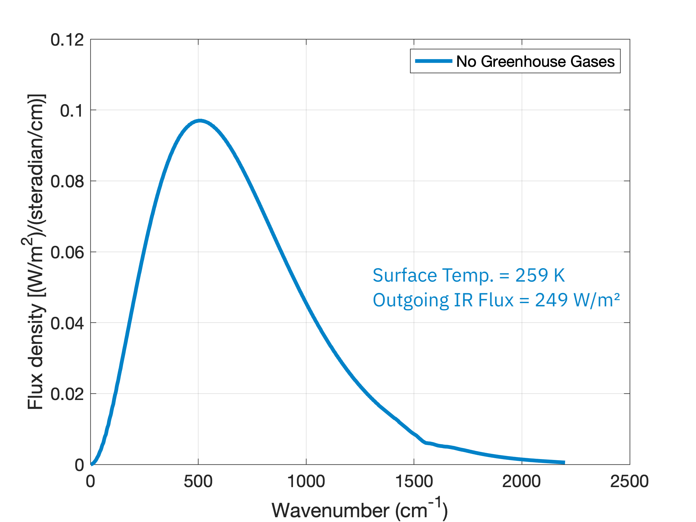
Notice that in this scenario the Earth’s surface is a frozen 259 K. If we add CO2 into the atmosphere at 415 ppm (the average 2022 level) and no other greenhouse gases, we see the missing emission chunk at the 667 \(\text{cm}^{-1}\) wavenumber and a large reduction in the radiation emitted to space, 221 \(\text{W}/\text{m}^2\), down from the original 249 \(\text{W}/\text{m}^2\):

Since the energy input from the Sun stays the same, the reduction in energy going out means energy will build up within the planet’s surface and atmosphere. However, this build up of energy can’t go on forever since that would violate physics’ second law of thermodynamics. So the atmosphere warms and thus emits more blackbody radiation just until it comes back into energy balance with what is coming in, 249 \(\text{W}/\text{m}^2\):
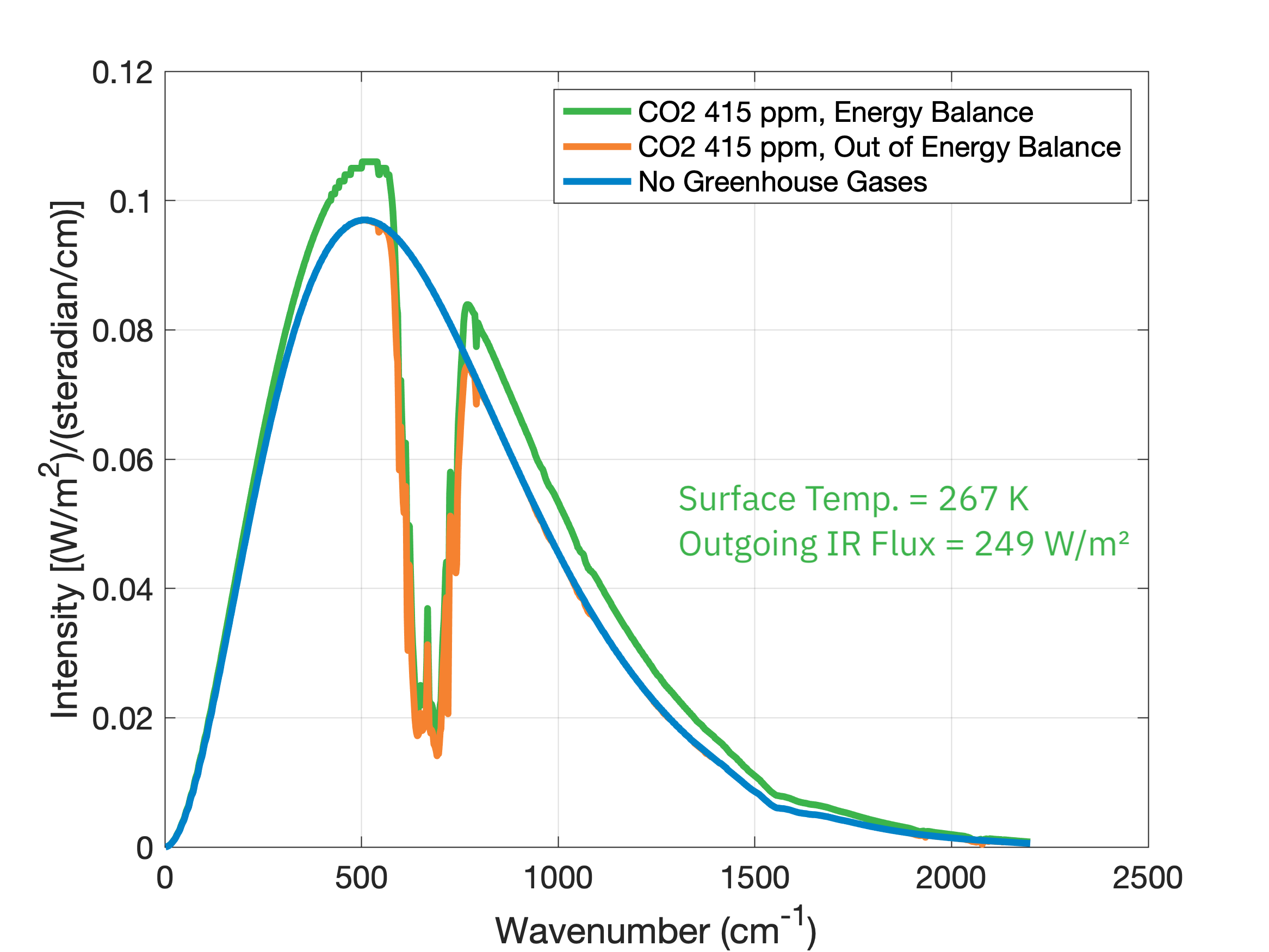
Notice that this warming has shifted the emission distribution upward, reflective of Earth's warmer temperature (267 K instead of 259 K). Mathematically, coming into energy balance means that the integrated area under the spectrum curve remains the same, so if we remove some of the area in one location we have to add more area in another. If we now put in all of the greenhouse gases currently present in Earth’s atmosphere and let the temperature and outgoing radiation adjust to energy balance, we get:
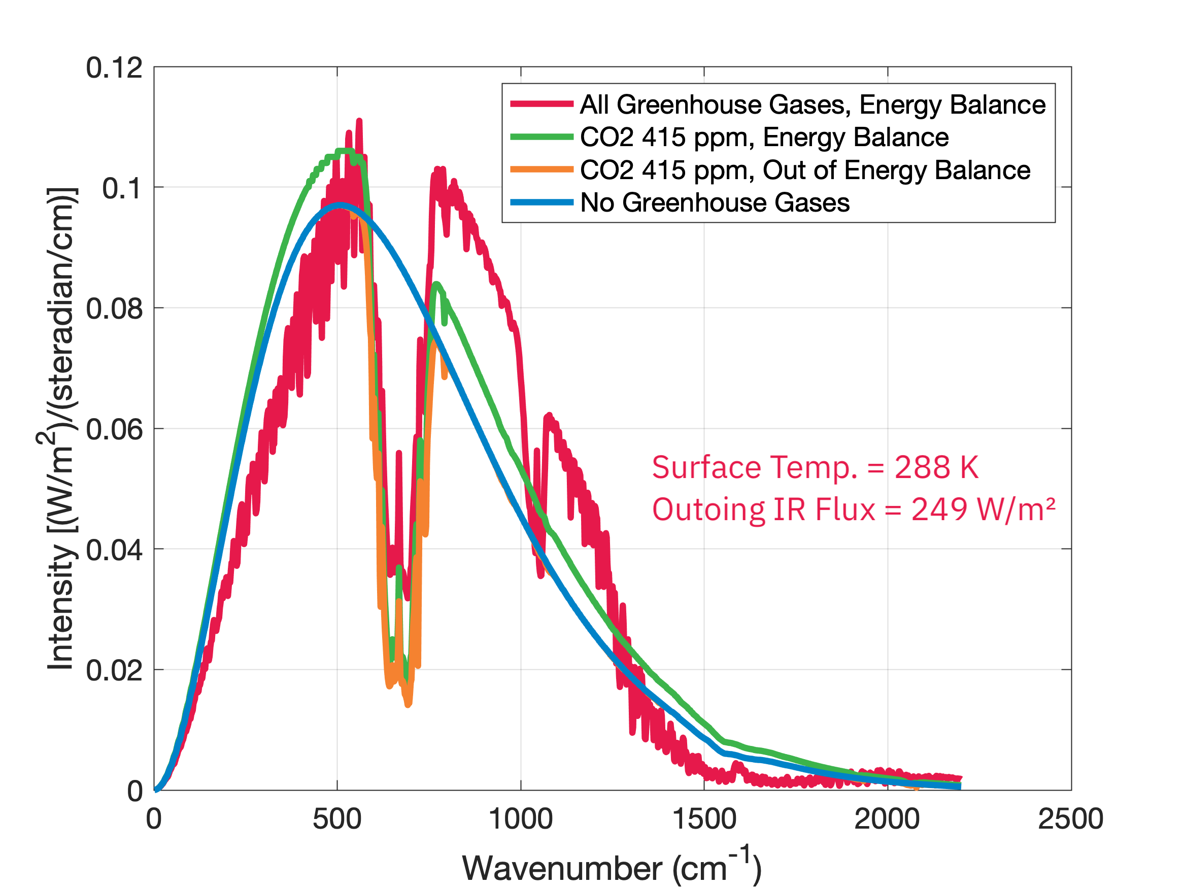
With the addition of even more greenhouse gases, we get even more radiation going down to the surface and a larger increase in surface temperature (up to the present-day 288 K) in order to balance energy coming in to the Earth system with energy going out. This is the radiative impact of Earth’s greenhouse effect.
Is it possible to completely saturate Earth’s atmosphere with greenhouse gases such that adding more won’t heat the surface of Earth? In the energy balance model we started the chapter with, this corresponds to increasing \(\epsilon\) until it equals 1; this limits the maximum warming in that model to \(T_s=302\, \text{K}\). The MODTRAN model we’ve used in this section is much more sophisticated than our simple energy balance model though. In these experiments we’ve progressively added more greenhouse gases to the atmosphere and we’ve seen that it simply radiatively adjusts: radiation in must balance radiation out and the temperature of the atmosphere warms to accomplish that. If we wanted to make the energy balance model more like the real atmosphere, we could add additional layers, each with their own pressure-dependent emissivity value. Then if you want to saturate the atmosphere with greenhouse gases, the problem is that the upper-most levels of the atmosphere will never get to sufficient pressure to have \(\epsilon=1\). The atmosphere of Venus is 96.5% CO2 and has a mass 94 times greater than Earth’s atmosphere. It’s surface temperature is an unbearable 737 K = 464°C. Adding even more CO2 to Venus’ atmosphere would just make it hotter.
\(\Uparrow\) To the top
\(\Rightarrow\) Next chapter
\(\Leftarrow\) Table of contents