Earth’s Atmosphere and Energy Balance
In the About section of this book, we motivated our journey with the following figure of global mean temperatures from observations and climate model simulations:
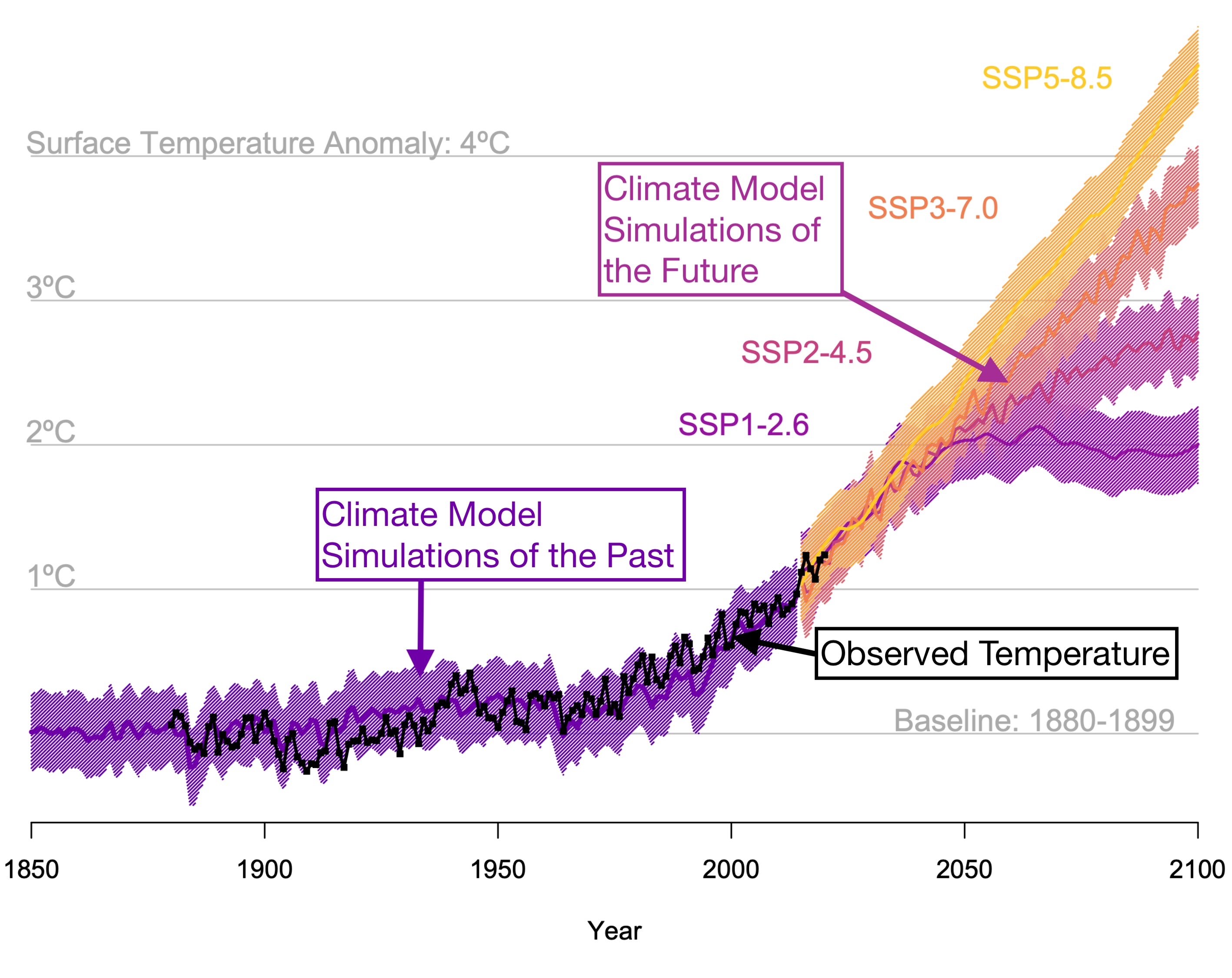
This chapter and the three others after it are the scientific explanation for why the globe has been warming, which you can see most clearly since about the 1970s. We begin this explanation with the atmosphere of Earth.
Earth’s Atmosphere
The atmosphere is big. Its total mass is \(5.1\times10^{18}\) kg, which is approximately the same mass as the Mediterranean Sea. The ocean as a whole is of course much more massive than the atmosphere, coming in at \(1.4\times10^{21}\) kg. Yet it is the atmosphere that largely controls the climate of Earth. Why is that? This section follows in outline Chapter 1 of Randall, Atmosphere, Clouds, and Climate, (2012).
The explanation has two parts. First, the atmosphere serves as an outer skin, standing between the other components of the climate system and space. As a result, the atmosphere can regulate the all-important exchanges of energy between the Earth and space, which take the forms of solar radiation coming in and infrared radiation going out (more about radiation below).
The second reason is that the atmosphere can transport energy and other things from place to place much faster than any other component of the climate system. Typical wind speeds are hundreds or even thousands of times faster than the speeds of ocean currents, which are in turn much faster than the ponderous motions of the continents.
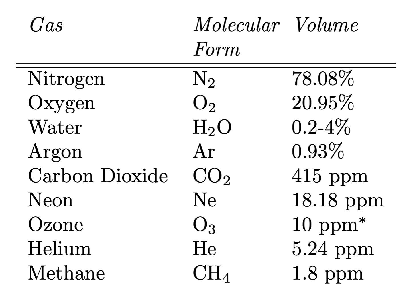
What is the atmosphere made of? The most abundant constituents of the atmosphere are the doubled elements of nitrogen (N2) and oxygen (O2). They are very well mixed throughout almost the entire atmosphere, so that their relative concentrations are essentially constant in space and time.
Ozone (O3) and water vapor (H2O) are ‘minor’ but very important atmospheric constituents that are not well mixed, because they have strong sources and sinks inside the atmosphere. Ozone makes up less than one millionth of the atmosphere’s mass, but that is enough to protect Earth’s life from deadly solar ultraviolet (UV) radiation. Water vapor is only about a quarter of 1% of the atmosphere’s mass, but its importance for the Earth’s climate, and for the biosphere, would be hard to exaggerate.
Carbon dioxide (CO2) is present in even lower quantities than ozone or water vapor. Yet, as we will discuss in more detail later, it turns out to also have a critical role in keeping Earth habitable. Similar to nitrogen and oxygen, carbon dioxide is well-mixed throughout the entire atmosphere.
Here is how the atmosphere varies with height in density, pressure, and temperature, from the surface to an altitude of 50 km, based on what is called the ‘U.S. Standard Atmosphere’:
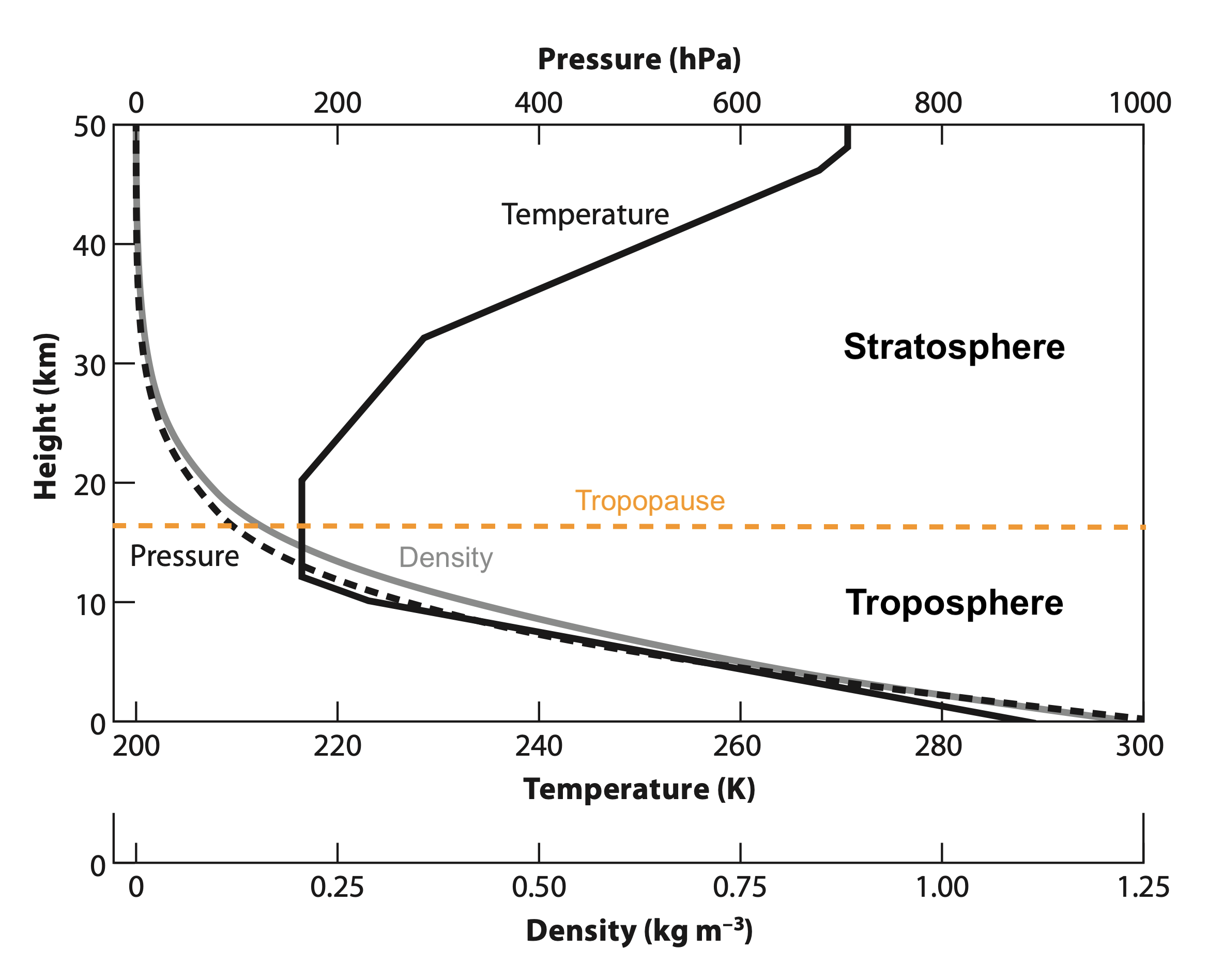
This figure shows the two lowest layers of Earth’s atmosphere. The troposphere at the bottom is where all of Earth’s weather takes place. The tropopause is the top boundary of the troposphere. At the top of this figure is the stratosphere, which is quite different than the troposphere. The stratosphere has basically no weather phenomena and increases in temperature with height instead of decreasing with height like the troposphere.
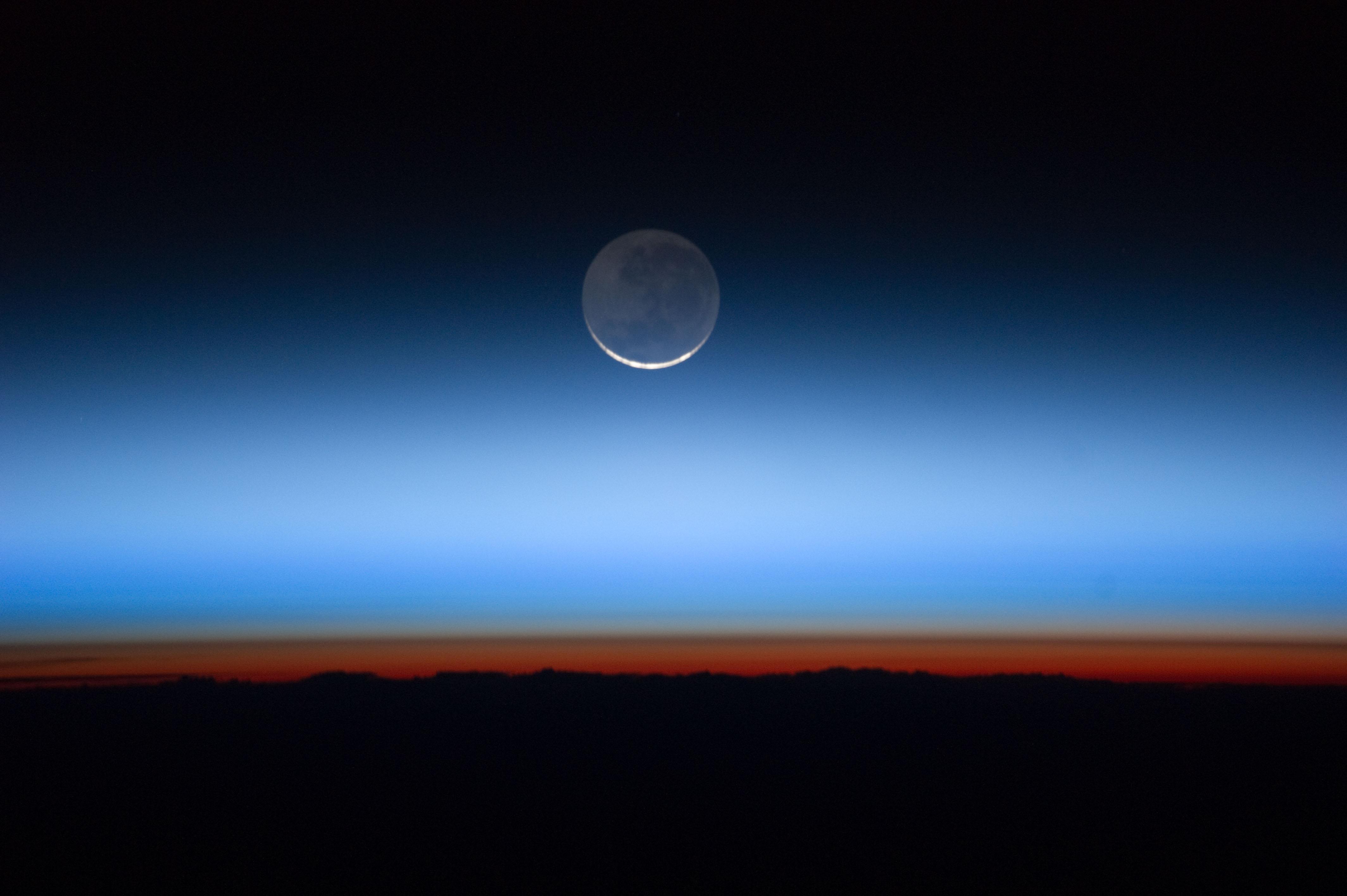
This viewpoint nicely shows what the layers of the atmosphere look like during a sunset from space, with red-orange colors indicating the troposphere and blue colors the stratosphere and upper atmosphere:
How heavy is a column of air? The total pressure is typically about 100,000 Pa or 1000 hPa near sea level (see figure above; 1 hPa = 100 Pa), where a Pa (pascal) is defined to be a newton (N) per square meter (or \(\text{Pa}=\text{N}/\text{m}^2 = \text{kg} / \text{m} \text{s}^2 \) ). For comparison, the weight of a typical car is about 20,000 N, so the weight of an air column per square meter is roughly equivalent to the weight of five cars piled on top of each other, over one square meter of a junk yard. That’s obviously pretty heavy.
As we saw in the ‘U.S. Standard Atmosphere’ figure, a dominant feature of the atmosphere is that the pressure decreases exponentially with height. In the ocean, pressure increases only linearly with depth. What explains the difference between the two?
To understand this, let’s first start with the basic physics of atmospheric gases. For atmospheres like the Earth that are not super dense and the gas is compressible, each gas approximately obeys the ideal gas law, where the pressure \(p\) for a particular gas can be written as \[p = \rho \frac{R}{\overline{M}}T \; , \tag{1}\] where \(\rho\) is the density of the gas, \(R\) is the universal gas constant, 8.314 J/(K mol), \(\overline{M}\) is the mean molecular weight of the gas, and \(T\) is the temperature. We can use this equation for any atmosphere as long as we know \(\overline{M}\) for whatever collection of gases are in it; for Earth, dry air has a mean molecular weight of 28.97 g/mol.
Equation (1) tells us how pressure varies as a function of temperature, but in order to explain how pressure varies with height in the atmosphere, we need to think about how vertical forces are balanced in the atmosphere.
We’ll need to balance the gravitational force going down with the force of the air pressure pushing back up. Consider a slice of a column of atmosphere that has a vertical thickness \(dz\) and a cross-sectional area \(A\) in the horizontal direction. Since pressure is simply force per unit area, \(P=F/A\), then the change in pressure from the base of this slice to the top of this slice is just the force exerted by the mass. Using Newton’s second law (force equals mass times acceleration) and balancing the two forces we have \[A dp=- g dm \; ,\] where \(g\) is the acceleration due to gravity (at sea level on Earth \(g = 9.80\, \text{m}/\text{s}^2\)), \(dm\) is the increment of mass in the column per unit area and the negative sign appears because the gravitational force points in the direction of decreasing \(z\). We can write this in terms of density as \[A dp=-A g \rho dz\] and dividing by \(dz\) to get the change of pressure with a change in height we get \[\frac{dp}{dz} = -\rho g \; .\tag{2}\] This equation is known as the hydrostatic equation and mathematically represents the dominant vertical force balance in the atmosphere.
How is this relationship different from water? Since water is not compressible, that means that its density is (approximately) constant even at great depths in the ocean. The force of the water pressure is just the force of the amount of mass of the water above a given depth \(D\). So \[p=\frac{F}{A}=g\frac{m}{A}=gD\rho_{water} \; . \tag{3} \] This gives us the linear relationship of pressure with depth for the ocean.
If we circle back to the original question that started this, how do we get an exponential decrease in pressure with height? If we combine Eq. (2) with the ideal gas law, Eq. (1), by substituting in for density \(\rho\) we get \[\frac{dp}{dz} = -\frac{p\overline{M}g}{R T}\; ,\] \[\frac{1}{p}dp = -\frac{\overline{M}g}{R T}dz\; .\] We can now integrate this equation, summing up all the infinitesimal air layers from the surface to the top of the atmosphere (assuming that T varies slowly with height and can be treated as a constant) to get \[p(z)=p_{s} \exp\left(\frac{-g \overline{M}z}{RT}\right) \; ,\tag{4}\] where \(p_{s}\) is the surface pressure of the gas. This equation shows the exponential decrease in pressure with height.
A puzzling feature of the atmosphere is that it warms throughout the stratosphere. What causes this? The answer lies in a series of chemical reactions. High energy UV light photons strike some of the O\(_2\) in the stratosphere and break it apart into two atomic oxygen molecules. The O atoms combine with molecular oxygen, O\(_2\), in the presence of other gas species, most often N\(_2\), to form ozone, O\(_3\). So these two processes create O\(_3\). O\(_3\) can be destroyed by being split apart by photons in one reaction and them combining with atomic O in another reaction to go back to O\(_2\). In these reactions it is the input of energy from photons that makes many of the atoms and molecules in these reactions move faster. From physics we know that temperature is really just a measure of the energy of the motions of atoms and molecules, so as the speed of the gases increase, so does the temperature. Thus the chemical production and destruction of ozone leads to a warm stratosphere.
The atmospheres of other planets can also have warm stratospheres if they have gases that behave similarly to oxygen and ozone on Earth, see below. For Jupiter, Saturn, Titan, Uranus, and Neptune, the stratospheric heating is due to methane (CH\(_4\)) and the heating of tiny particles suspended in the air called ‘aerosols’.

Physics of Radiation
The most familiar source of energy warming a planet is the absorption of light from the planet’s star. This is the dominant way that Earth and other rocky planets like Venus and Mars are heated. It’s also possible to heat the surface of a planet from below. Heat can come up from the interior of a planet due to radioactive decay, massive gravitational tides (tidal dissipation), or hot material left over from the formation of the planet. Relative to the amount of sunlight they absorb, heat flux from below the surface of the planet is important for the ‘surface’ climates of Jupiter and Saturn but not for rocky planets like Earth. Gas giants can transport heat from their interiors through the motions of gases in their atmospheres. But on a rocky planet like Earth the diffusion of heat is sluggish through the solid rock, so the deep interior heat contributes only a tiny amount to the surface temperature of Earth. Pierrehumbert, Principles of Planetary Climate, 2010.
While there are many ways a planet can gain energy, there is essentially only one way a planet can lose energy. Since a planet sits in the hard vacuum of outer space, and its atmosphere is rather tightly bound by gravity, not much energy can be lost through heated matter streaming away from the planet. The only significant energy loss occurs through emission of electromagnetic radiation. Pierrehumbert, Principles of Planetary Climate, 2010. Electromagnetic radiation is the historical term given to all the different kinds of photons: visible light, gamma ray, x-ray, ultraviolet, infrared, microwave, and radio; these are all photons, which are wave-like packets of energy that travel at the speed of light. These photon types are equivalently called ‘electromagnetic radiation’ or ‘electromagnetic waves’ or simply ‘radiation’ but each type has a different range of wavelengths and energies.
Here is how the different kinds of radiation relate, lined up next to each other according to wavelength and frequency, along with a closer look at an example visible blue light photon on the bottom of the figure:
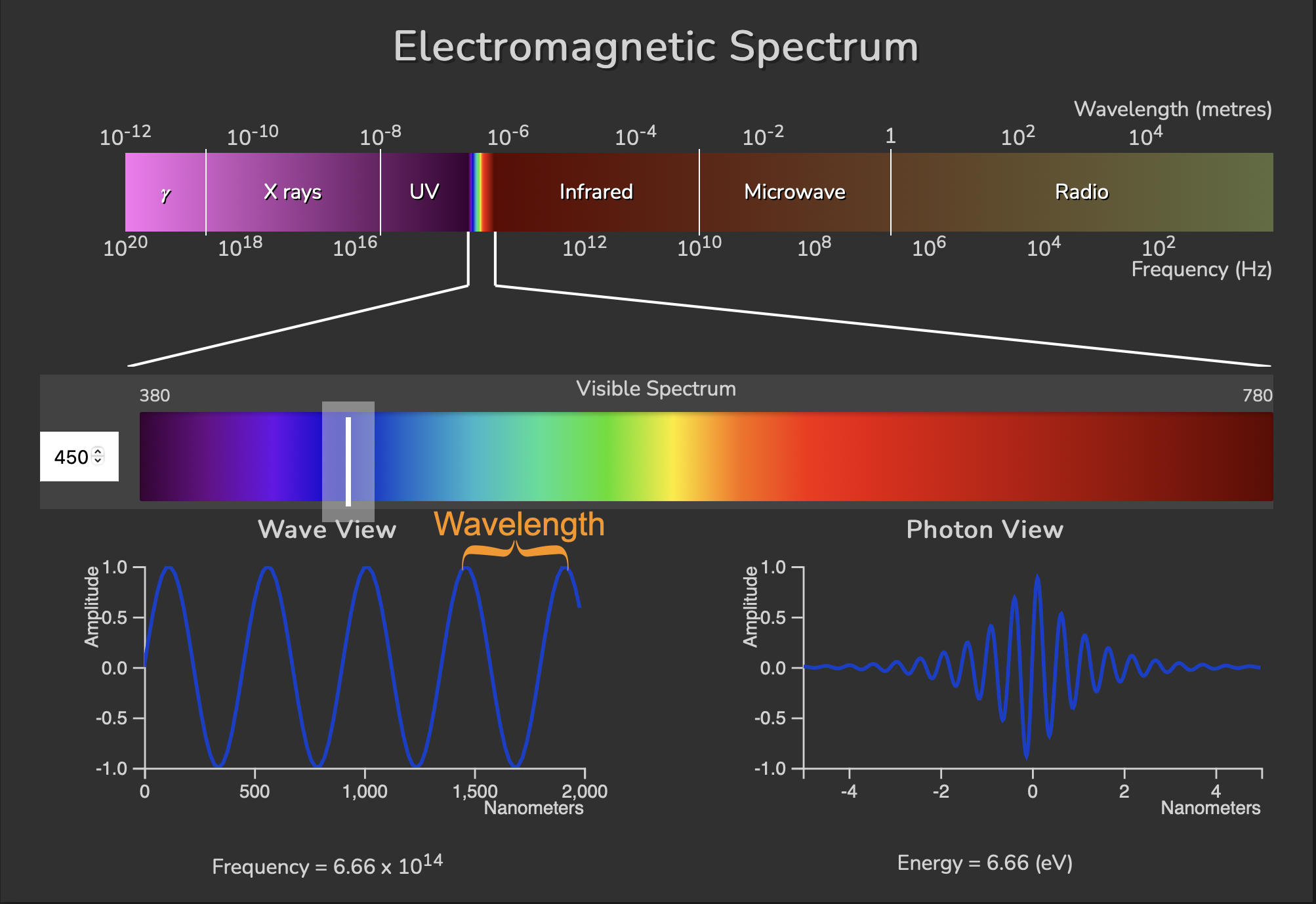
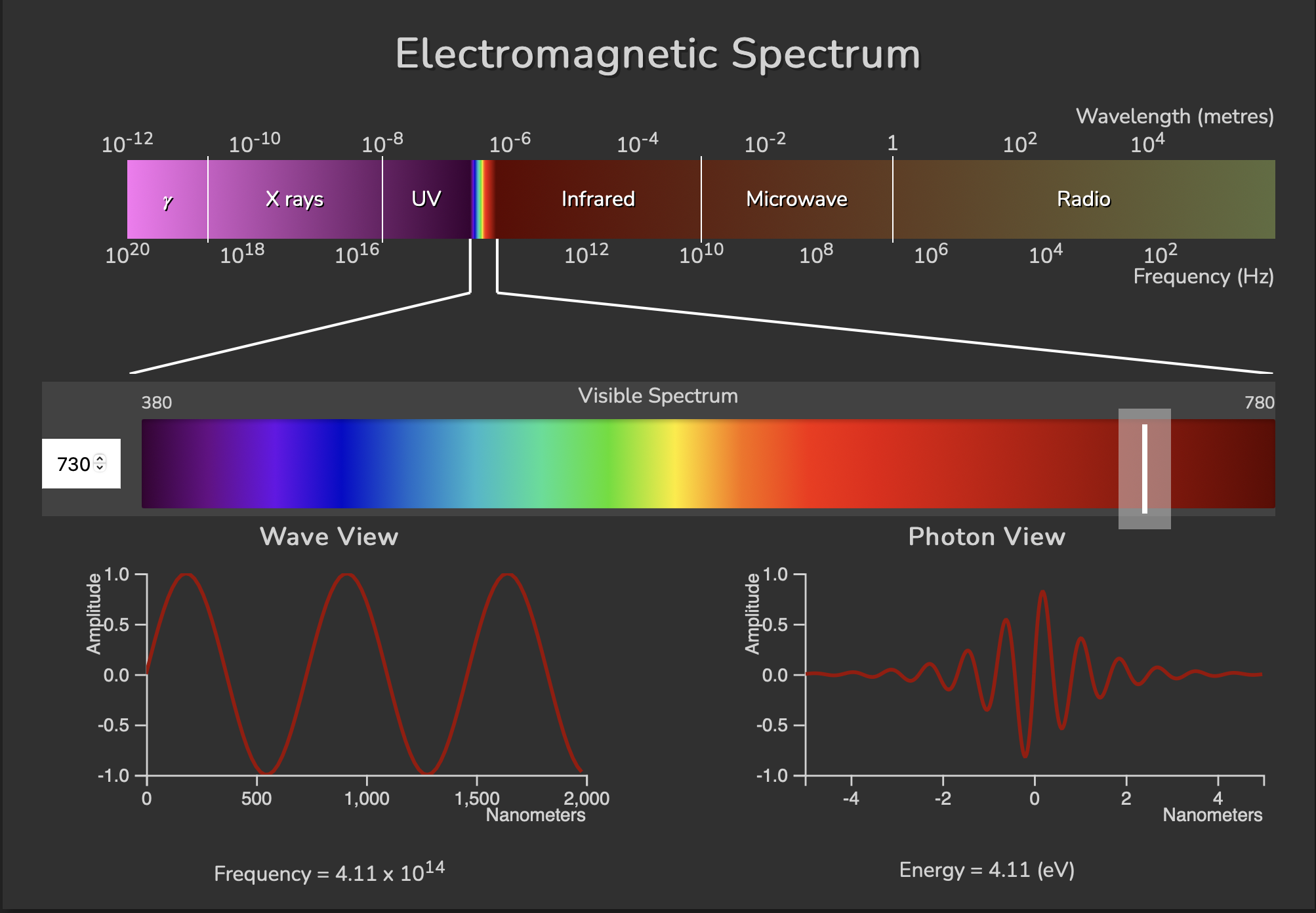
On the bottom we’re picking out a blue light photon with a wavelength of 450 nm. The wavelength is the distance from one peak to another if we think of a stream of photons behaving like a long wave. Photons individually act like a wave packet of energy, illustrated on the bottom right ‘Photon View’. A photon wavelength \(\lambda\) is related to its frequency \(\nu\) by the speed of light \(c\) through the equation: \(\lambda = c/\nu\). This equation tells us that if we increase the wavelength, the frequency will decrease. We can also see this if we compare the blue light example to a red light (730 nm wavelength) example below. The red light has a longer wavelength and a decreased frequency:
We know from experience that something that is heated to a very high temperature glows red or white, thus emitting visible photons or electromagnetic radiation. Similarly, almost any object that has a temperature at all, also emits electromagnetic radiation (though at typical Earth temperatures it is radiation that we cannot see). This phenomena is called ‘blackbody radiation’. Blackbody radiation is incredibly important in the history of physics. In the process of figuring out a mathematical description of this phenomena, the physicist Max Planck accidentally discovered the foundational idea of quantum mechanics: that radiation is emitted only in small packets of energy, called at the time ‘quanta’. Specifically, the quantum of energy for radiation having frequency \(\nu\) is \(E=h\nu\), where \(h\) is known as ‘Planck’s constant’. This energy value, in units of electronvolts (eV), is what is shown in the bottom right ‘Photon View’ panels of the blue and red light figures above. The size of \(h\), which is equal to \(6.626\times 10^{-34}\) Joule-seconds, determines the granularity of reality. This value is so small that we don’t notice quantum effects in everyday life.
After discovering the energy-quanta idea, Max Planck derived an equation for how an object would emit radiation, now known as the ‘Planck function’, \[ B(\nu,T) =\frac{2h\nu^3}{c^2}\frac{1}{e^{h\nu/kT}-1}\; , \tag{5}\] where \(B(\nu,T)\) is the irradiance or flux emission spectrum. Here’s what the Planck function looks like for different temperature values (in degrees K):
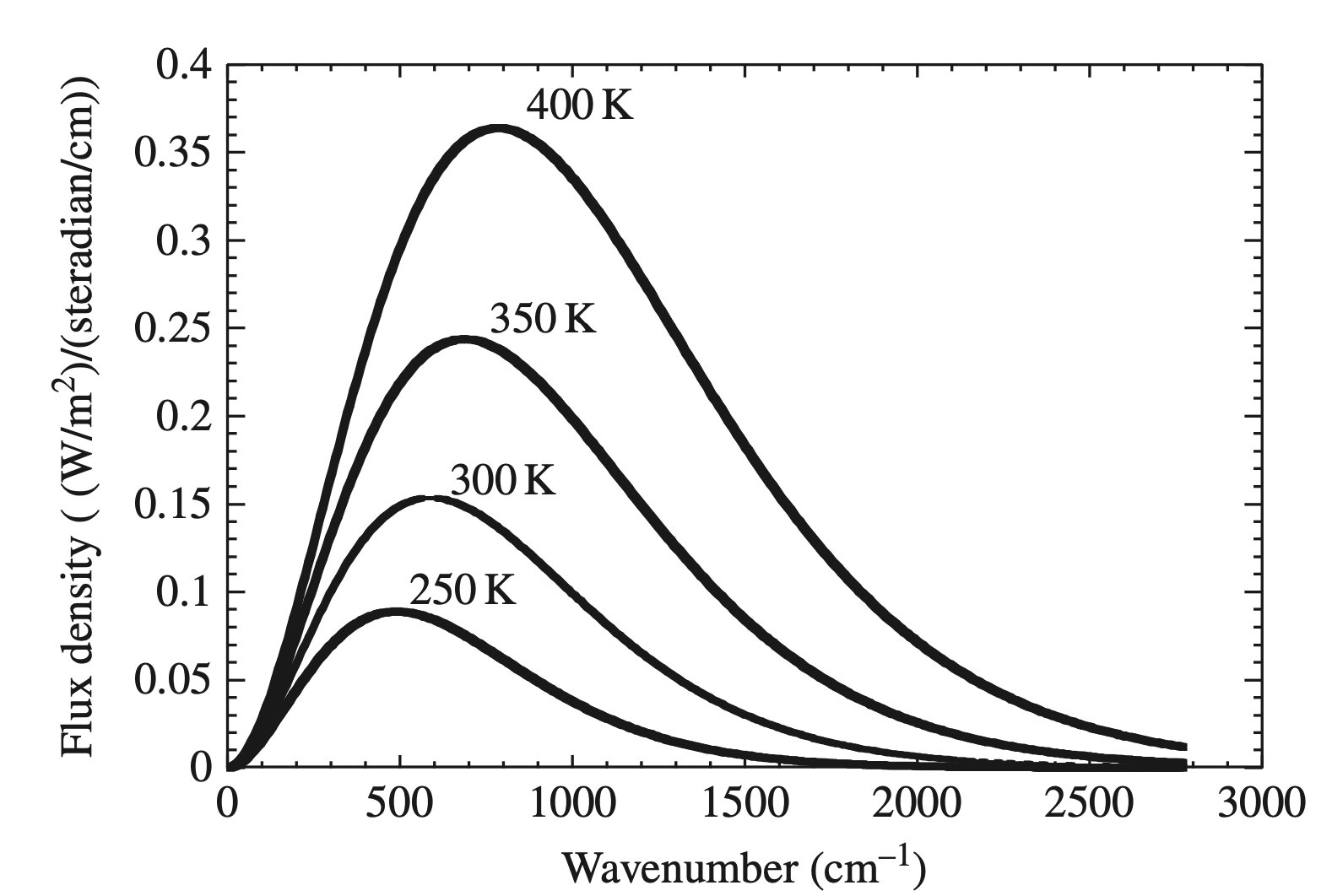
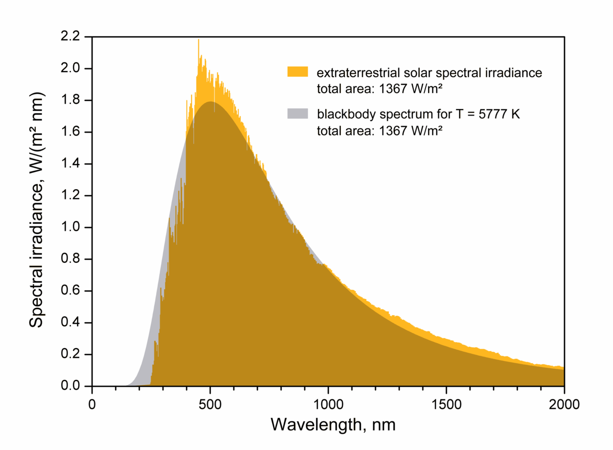
The Plank function shows you the distribution of radiation that is emitted for a perfect ‘blackbody’ at a given temperature, plotted above as a function of wavenumber (the inverse of wavelength, \(1/\lambda\)). A perfect blackbody is an object with a rich energy spectrum that can emit (or absorb) all frequencies of radiation. By musical analogy, a ‘blackbody instrument’ would be a hypothetical musical instrument that could play every possible note, instead of a small range like normal instruments. A ‘black’-body is named that way for historical reasons related to the theoretical idea behind how it was mathematically derived. In reality many things behave very similarly to blackbodies but aren’t very black at all, such as planets and stars. Below is a figure showing that the sun’s emission spectrum (yellow) compares fairly well to a perfect blackbody Planck function (gray).
Nearly all objects radiate photons, but not all objects emit them according to a blackbody distribution. One example is the emission spectra of many galaxies. Take for example the emission spectrum of the irregular galaxy NGC 6052, composed of a group of stars and gas (Sloan Digital Sky Survey III Science Archive Server, accessed Feb 2022).
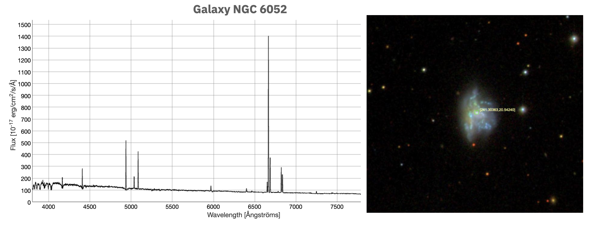
This galaxy clearly shows emission lines instead of a basically smooth Planck distribution. This is because the emission spectrum we are seeing is primarily from the heated gas between the stars of the galaxy. And gases by themselves emit photons for only specific wavelengths related to their atomic structure. Here we are seeing emission lines predominantly from the gases hydrogen and helium.
It’s very useful to know what the total power output of a blackbody is (where power is energy per unit time). To find an equation for that power \(\mathcal{F}\), we can assume a spherical object and integrate the Planck function over all frequencies, \[\mathcal{F} =\int^{\infty}_{0} \pi B(\nu,T) d\nu =\int^{\infty}_{0}\frac{2\pi h}{c^2}\frac{\nu^3}{e^{h\nu/kT}-1}d\nu =\sigma T^4 \; ,\tag{6}\] where \(\sigma = 2\pi^5k^4/(15c^2h^3) \approx 5.67\times 10^{-8} \text{W}/(\text{m}^2\text{K}^4)\) is known as the Stefan-Boltzmann constant. This equation, \(\mathcal{F}=\sigma T^4\), is called the Stefan-Boltzmann law. We will use this law to derive simple climate models for a rocky planet like Earth.
Earth’s Energy Balance
As we discussed previously, the surface of Earth is heated almost entirely by the Sun. The incoming solar radiation gets spread across the surface of the Earth and is balanced by Earth’s outgoing radiation. This fundamental situation is referred to as Earth’s planetary energy balance.
In order to figure out the precise amount of solar radiation Earth receives, we need to work out some geometry. Because the Sun is so far away, solar photons come in almost exactly parallel to each other. As the Earth rotates, this solar radiation, \(S\), is absorbed across the entire surface area of Earth. If we assume that Earth is perfectly spherical and has a radius \(a\), then this surface area is \(4\pi a^2\). Yet the solar radiation that Earth receives is the amount that would hit a disk with the same radius as Earth. This energy balance and geometrical situation is sketched out below:
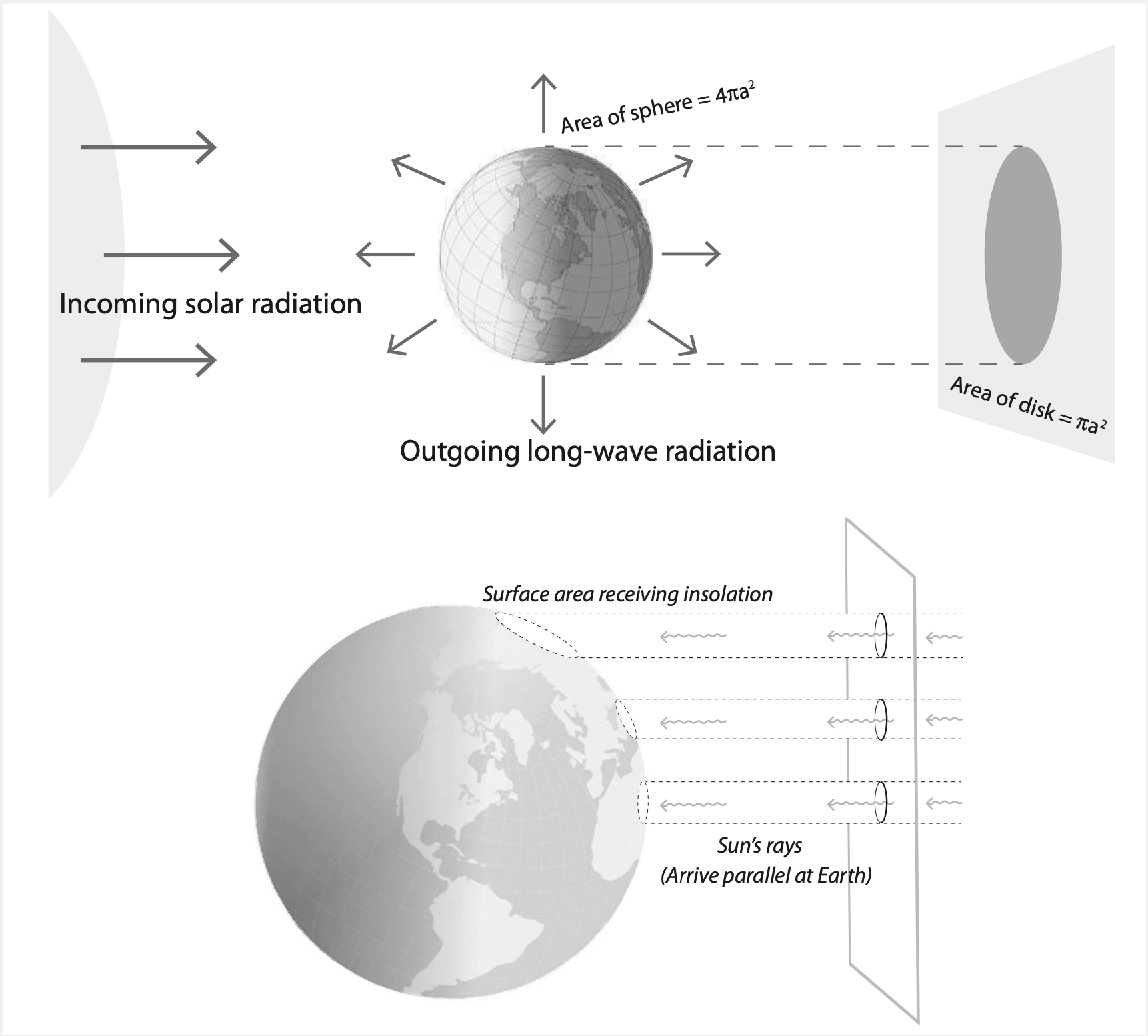
The incoming solar radiation that hits the ‘Earth disk’ is \(S\pi a^2\) and this gets divided over the surface area of Earth. So the total solar radiation is \(S\pi a^2/(4\pi a^2)=S/4\), where \(S=1361 \text{W}/\text{m}^2\) at Earth’s orbital distance.
As we worked out previously, we know that a planetary blackbody like Earth will emit radiation to space following the Stefan-Boltzman law, \(\mathcal{F}=\sigma T^4\). If the Earth were to absorb all solar radiation, then the energy balance of Earth can be written as \(S/4=\sigma T^4\). In actuality, the energy balance isn’t quite this simple since some solar radiation gets reflected back out to space before it has a chance to be absorbed by the Earth. This reflected amount of radiation is called the ‘albedo’, denoted by \(\alpha\). Earth’s global average albedo is approximately 0.31. Planets in the solar system have albedos that range from Mercury’s 0.07 all the way up to 0.77 for the cloudy and reflective Venus. So correcting for albedo, we have an energy balance equation of \[\frac{S}{4}(1-\alpha) = \sigma T^4 \; .\tag{7}\] If we solve this equation for \(T\) and plug in the constants we find that Earth’s temperature ought to be \(T=253.7\, \text{K} = -19.5 ^{\circ}\text{C}\). Obviously something has gone wrong here since Earth isn’t a frozen snowball! This is the simplest, basically accurate model of global climate that exists, yet we see here that it is in fact too simple. This model of Earth’s climate has neglected the atmosphere and its greenhouse effect, which will be the subject of our next chapter.
\(\Uparrow\) To the top
\(\Rightarrow\) Next chapter
\(\Leftarrow\) Table of contents